My Finance

0. First Remarks. We need to use the Yeo-Johnson transform, not the Box-Cox transform to make data normal, since we need to ensure data can be both positive and negative. When we run modified random walk and autoregression simulations, we can always get outside of set bounds where the inverse Box-Cox transform is defined. We succeeded in this. And we can run simulations of such transformed volatility, and transform it back using the inverse Yeo-Johnson transform, no problem.

First, we must transform log volatility, then fit the autoregression. We should not first fit the autoregression for log volatility, then transform the residuals. This would give us IID Gaussian data, but will not allow us to make objective Bayes inference for linear regression. Transforming the original data first allows us to simulate regression coefficients and standard errors.

The code and data are given in this new GitHub repository.

1. Simulation Description. We fit a one-factor model for stock returns (nominal, total, geometric) for three asset classes:

• US stocks (domestic, measured by S&P 500)
• International developed markets (measured by 88% MSCI EAFE + 12% MSCI Canada)
• International emerging markets (measured by MSCI EM)

Of course, for the latter two, we have less data: 1927-2025 for US stocks, 1970-2025 for developed, and 1988-2025 for emerging. Therefore, we expect Bayesian inference to make a difference. For each of 3 classes, we have two choices:

• Keep volatility original, as is
• Apply the Yeo-Johnson transform

We apply three modes of statistical inference, following this blog post:

• Classic (frequentist, with point estimates for the covariance matrix of innovations and regression coefficients)
• Bayesian lite (fixed covariance matrix for innovations, objective Bayes posterior for regression coefficients)
• Bayesian full (fixed correlation matrix for innovations, objective Bayes posterior for standard errors and regression coefficients)

For each of the 18 experiments, we run 10000 Monte Carlo simulations for 20 years. We return 10 results:

• For average returns over 20 years, mean, stdev, and percentiles 10, 30, 50 (=median), 70, and 90.
• For 3%, 4%, 5% withdrawal rules with 4% annual arithmetic increase to adjust for inflation, the ruin probability.

2. Conclusion. We do not see much difference in ruin probability. But a lot of difference in lower quantiles and in the median. However, not much difference between Bayesian-lite and Bayesian-full. Therefore, later we simply consider Bayesian-lite mode as an alternative to the frequentist approach.

Why do we need to simulate the objective Bayes posterior for the standard error? Instead, we can simply treat it as fixed, using the point estimate (in the same way as we do for the correlation matrix)? It is much easier to simulate only regression coefficients using the objective Bayes posterior. The latter coincides with classic frequentist confidence regions and intervals. Equivalent to fixed correlation matrix and standard errors is fixed covariance matrix.

3. Tables of results. Here we have complete tables which corroborate the conclusion in Section 2.

American stocks without and with the Yeo-Johnson transformation of log volatility, in %.

Statistic	Frequentist Original	Bayesian-lite Original	Bayesian-full Original	Frequentist Transformed	Bayesian-lite Transformed	Bayesian-full Transformed
Average	9.20	9.05	9.05	9.00	8.72	8.71
Stdev	4.29	5.23	5.26	4.85	6.45	6.44
Median	9.54	9.63	9.65	9.56	9.58	9.62
10%	3.53	2.54	2.36	2.97	1.64	1.47
30%	7.30	6.93	7.01	7.14	6.75	6.78
70%	11.62	11.99	11.96	11.72	12.04	12.00
90%	14.29	15.02	15.11	14.79	15.16	15.19
3% ruin	16	19	19	18	21	21
4% ruin	25	28	27	26	29	28
5% ruin	35	37	37	36	37	37

Developed stocks without and with the Yeo-Johnson transformation of log volatility, in %.

Statistic	Frequentist Original	Bayesian-lite Original	Bayesian-full Original	Frequentist Transformed	Bayesian-lite Transformed	Bayesian-full Transformed
Average	6.84	6.60	6.63	6.50	6.00	6.04
Stdev	5.64	7.42	7.39	6.56	9.52	9.40
Median	7.36	7.61	7.55	7.41	7.54	7.52
10%	-0.57	-2.53	-2.71	-1.64	-4.13	-4.26
30%	4.33	3.83	3.86	4.08	3.46	3.53
70%	10.08	10.74	10.79	10.21	10.87	10.93
90%	13.58	14.84	14.85	13.74	14.98	15.01
3% ruin	34	36	36	35	36	37
4% ruin	49	45	45	45	45	45
5% ruin	55	53	53	54	52	53

Emerging stocks without and with the Yeo-Johnson transformation of log volatility, in %.

Statistic	Frequentist Original	Bayesian-lite Original	Bayesian-full Original	Frequentist Transformed	Bayesian-lite Transformed	Bayesian-full Transformed
Average	8.55	8.29	8.33	8.21	7.69	7.75
Stdev	7.08	9.89	9.86	8.04	12.31	11.61
Median	9.15	9.34	9.34	9.18	9.35	9.31
10%	-0.72	-3.82	-4.27	-1.74	-5.26	-5.97
30%	5.46	4.47	4.42	5.18	4.16	4.13
70%	12.58	13.67	13.80	12.70	13.78	13.85
90%	16.97	19.33	19.72	17.13	19.51	19.83
3% ruin	32	35	35	67	36	36
4% ruin	41	42	42	59	42	42
5% ruin	48	48	48	48	47	48

4. Verification. The content of this section is taken from the file vol-transform.py The transformed log volatility is Gaussian, unlike the log volatility before the transformation. The is the parameter for the transformation.

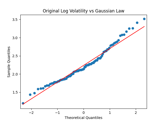
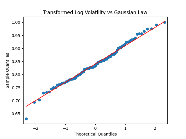
Below we see the quantile-quantile plot of autoregression residuals The regression fit is with Shapiro-Wilk and Jarque-Bera normality tests for give us and respectively.

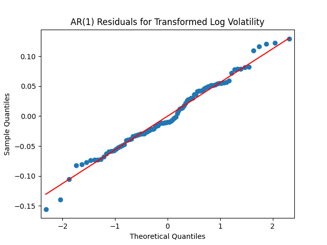
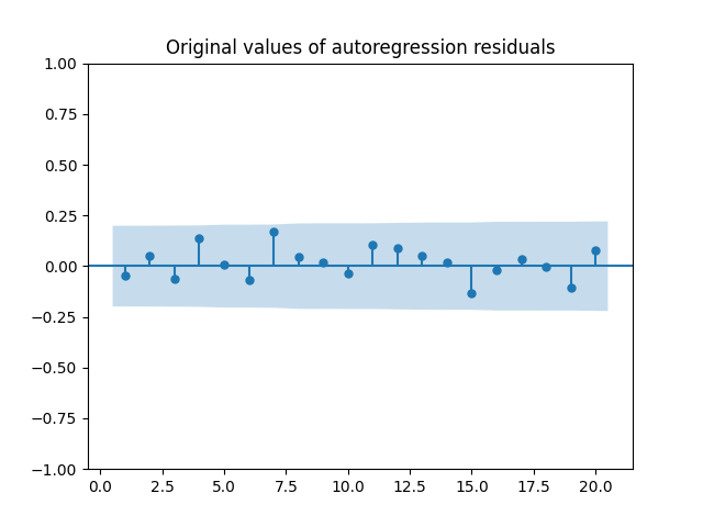
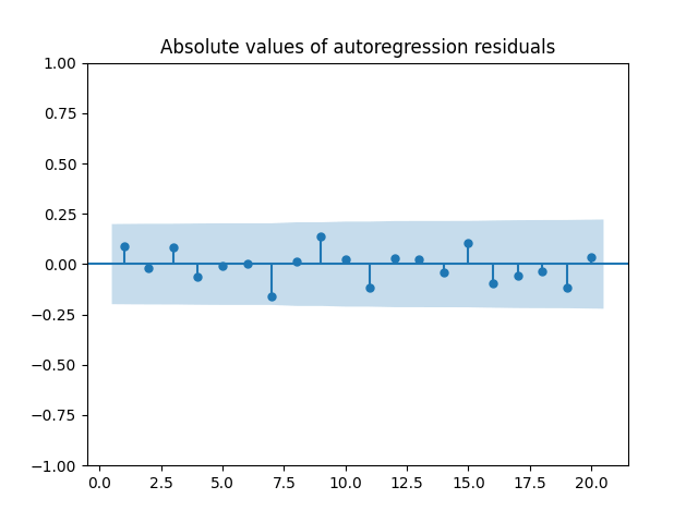
And we see the autocorrelation function for original and absolute values of autoregression innovations. We see that they are well modeled by IID Gaussian random variables.

5. Updates. Apologies, I absolutely forgot that series of the two innovations also need to be correlated. All this was done for two independent series of residuals. But we still benefited from it, since we made this mistake for both original and transformed data; and for classic vs Bayesian. We need to include covariance matrix of innovations, for both classic and Bayesian versions.

Below we provide the three tables for domestic, developed, emerging stocks. Compare them with Section 3.

US stocks, measured by S&P 500, with correlated innovations.

Statistic	Frequentist Original	Bayesian-lite Original	Bayesian-full Original	Frequentist Transformed	Bayesian-lite Transformed	Bayesian-full Transformed
Average	8.1	7.8	7.9	7.7	7.2	7.1
Stdev	4.7	5.7	5.7	5.6	7.5	8.6
Median	8.6	8.6	8.6	8.5	8.4	8.5
10%	2.0	0.5	0.7	0.7	-1.1	-0.9
30%	6.1	5.6	5.7	5.7	5.1	5.3
70%	10.8	11.1	11.1	10.8	11.1	11.1
90%	13.8	14.4	14.4	13.9	14.4	14.4
3% ruin	23	26	25	25	28	27
4% ruin	33	35	34	35	37	36
5% ruin	43	44	44	44	45	45

Developed international markets, measured by 88% MSCI EAFE + 12% MSCI Canada, with correlated innovations.

Statistic	Frequentist Original	Bayesian-lite Original	Bayesian-full Original	Frequentist Transformed	Bayesian-lite Transformed	Bayesian-full Transformed
Average	6.1	5.6	5.6	5.6	4.8	4.6
Stdev	6.1	7.9	8.2	7.2	10.3	16.4
Median	6.7	6.8	6.7	6.6	6.7	6.7
10%	-1.9	-4.5	-4.6	-3.5	-6.6	-6.4
30%	3.4	2.7	2.7	3.0	2.2	2.4
70%	9.6	10.2	10.2	9.7	10.3	10.2
90%	13.3	14.4	14.5	13.5	14.4	14.6
3% survival	39	40	40	40	41	41
4% survival	49	49	49	49	50	49
5% survival	58	58	57	58	57	57

Emerging markets, measured by MSCI EM, with correlated innovations.

Statistic	Frequentist Original	Bayesian-lite Original	Bayesian-full Original	Frequentist Transformed	Bayesian-lite Transformed	Bayesian-full Transformed
Average	6.6	9.05	6.1	5.9	5.1	4.9
Stdev	8.0	5.23	11.0	9.4	13.7	19.3
Median	7.3	9.63	7.6	7.3	7.4	7.4
10%	-3.8	-7.8	-7.8	-5.8	-10.0	-9.8
30%	3.2	2.0	1.9	2.6	1.4	1.6
70%	11.2	12.6	12.4	11.3	12.2	12.3
90%	16.1	18.1	18.2	16.3	18.2	18.4
3% ruin	41	43	42	42	43	44
4% ruin	49	50	49	50	50	50
5% ruin	56	55	55	56	55	56

We see that making residuals correlated makes values at risk for 10% and 30$ even more biased downward, especially for the international markets, where we have less data. Doesn’t it contradict the diversification principle, which states we need to ivnest even in riskier assets, when they are not well correlated with the benchmark? Turns out if there is not enough observations for these risky assets, then this uncertainty in parameter estimates outweighs the variance reduction.