My Finance

0. Introduction. I remembered we can apply the Box-Cox transform to make the data closer to normal. We can do this either with regression inputs, or regression outputs, or regression residuals. The data does not have to be IID. The main goal is to make new regression residuals Gaussian.

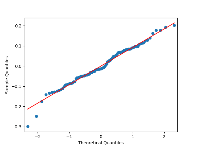
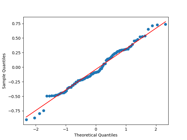
1. The annual volatility. This works very well for annual volatility data, both for raw data and autoregression residuals which are proved to be IID. See the Python code in the same GitHub repository for the current version of the simulator. See the resulting quantile-quantile plots for the transformed volatility; and for the transformed residuals for autoregression of the original log volatility.

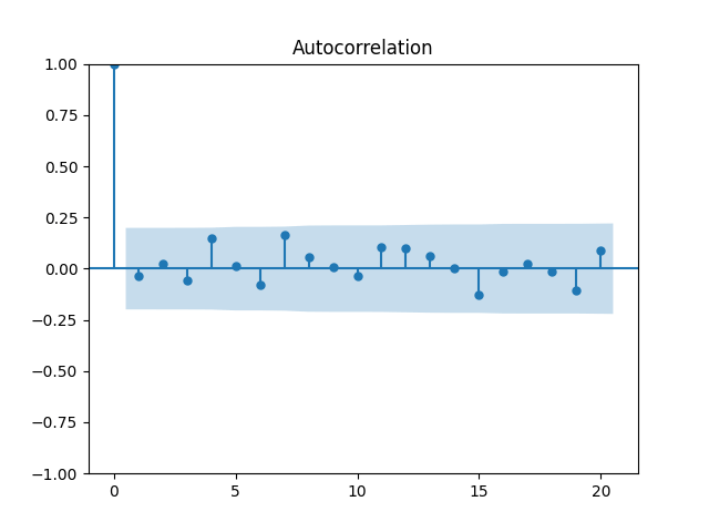
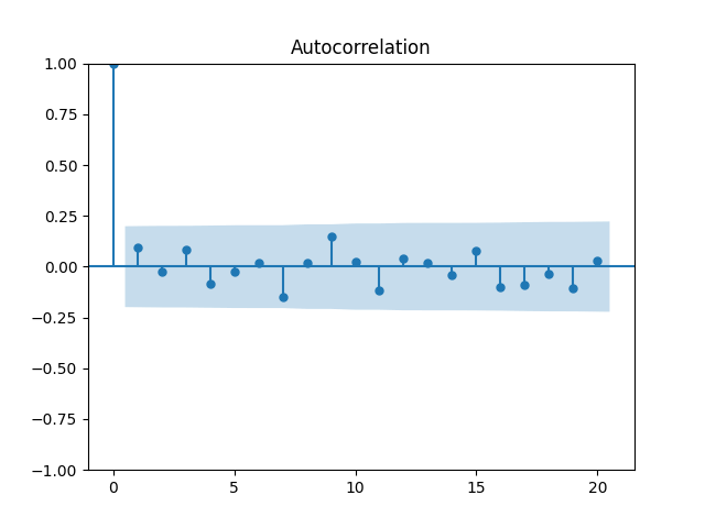
See also the autocorrelation function plots for original and absolute values of autoregression residuals for transformed volatility. These are very consistent with being independent identically distributed.

For the Box-Cox transforms of the residuals for the autoregression of original log volatility, we do not need to check that they are independent identically distributed, because we already checked this for these residuals. The normality tests (Shapiro-Wilk and Jarque-Bera) have I think it is better to transform volatility instead of residuals. The index in this Box-Cox transform is -0.594.

2. Other residual series for the current simulator. Consider the non-Gaussian series of residuals from the same repository of the current simulator. They are for Do not forget to exponentiate these residuals, since we need positive data for the Box-Cox transform. The other three regressions have Gaussian residuals, and they are all for asset classes returns. We already discussed the volatility. Judging by the Shapiro-Wilk and Jarque-Bera normality tests, we succeeded in making Gaussian the series for and but failed for and We see this in the file in the same repository.

3. Other data series for the current simulator. Consider the series of data themselves, rather than their residuals: To each apply the Box-Cox transform and then test Gaussianity. We succeed for but fail for Later, fit the autoregression of order 1 to the transformed data, and test innovations for IID Gaussian. We fail for all three series! Such a miserable failure to replicate our results but make them Gaussian. A reminder: We can apply the Box-Cox transform to data for the autoregression and only then fit this autoregression; or to its residuals after fitting the autoregression with original data. Unfortunately, we succeeded only in one case: making Gaussian (and IID) residuals for the BAA rate. This is done in this file in the same repository.

4. Exponentiated total log returns for three asset classes. The data for the Box-Cox transform needs to be positive. This cannot be said for log returns for US stocks, international stocks, and corporate bonds, so we exponentiate each of them. The Box-Cox transform, miraculously, transforms each of them into a sequence of IID Gaussian data. Fantastic! This is also done in the file in the same repository.

5. Implications. Remember, our goal is to construct a financial simulator with only Gaussian innovations. In part, because we wish to apply Bayesian analysis there. As is clear from Section 1, we succeeded here, except the borderline case of stock volatility.

But, helpfully, this Box-Cox transform gives us a way out: Just transform the volatility and run the autoregression. This enables us to build a version of our simulator which has indeed only Gaussian innovations. Let us call this Version O.

Another version would be simple, with only asset classes (including maybe emerging stocks, check!) and without volatility at all, the only factor is BAA rate. As discussed above in Section 3, we can transform residuals of the autoregression for log rates to make them Gaussian. Let us call this Version R.

Also, we can include the volatility as in the Version R, and combine this with the BAA rate. This would be Version V.

Finally, we can remove the volatility from the Version O, and apply the Box-Cox transform to these asset class returns. This would be Version C.

None of the versions include long-short spread, and earnings growth. Unfortunately, we cannot transform the current version of the financial simulator into a version with Gaussian innovations.

But we can transform the simple version into the one with Gaussian innovations. This would be Versions R or V. Do not forget to check emerging stocks! Also, we can transform (after checking for emerging stocks!) the newest version, this would be Versions C or O.

6. Stock Returns. I checked log returns of each of three stock asset classes: USA, developed, emerging. For each, I took both the original data and normalized by volatility. For both cases, I took the data itself and after the Box-Cox transform. I applied to each of the resulting 12 series the following tests: Shapiro-Wilk, Jarque-Bera (for normality) and Ljung-Box for 5 and 10 lags for original and absolute values of residuals (for IID).

Outcome: I think it is better to either normalize or transform the returns data, but not both. Better normalize, since this works for all three asset classes. But can we really apply the normality tests on such small sample size, only 1988-2025 (38 data points) for emerging stocks? I am not sure.

US stocks: All pass all tests, except the original (non-normalized and non-transformed) data, which is IID but not Gaussian.

Developed markets: Same as the US stocks.

Emerging markets: All pass all tests, except the Ljung-Box test for original values of 10 lags.

• Original data has
• Normalized has
• Transformed has
• Transformed normalized has

See the Python file in the newest repository. The best models seem to me now Versions O or V.