New Valuation Measure Replicated + Volatility

Background: I continue the previous post of joint work with my undergraduate student Angel Piotrowski. Consider my work arXiv:1905.04603. We wrote about this in yet another post. In a GitHub/asarantsev repository we updated our code and data.

Let  E(t) be the 10-year trailing averaged annual real earnings. Let  G(t) = \ln(E(t)/E(t-1)) be the log growth terms. We compute these for  t = 1928, \ldots, 2024. Also, let  Q(t) be total real returns for the same years. Then  \Delta(t) = Q(t) - G(t) is implied dividend yield; we assume  c is its long-term average. We model the valuation measure  H(t) = \Delta(1) + \ldots + \Delta(t) - ct as an autoregression of order 1:

 H(t) - h = b(H(t-1) - h) + Z(t),

where innovations  Z(t) are independent identically distributed, with mean zero.

As discussed before, the difference between our research and arXiv:1905.04603 is that we take December CPI data instead of January to compute inflation, and end-of-year S&P index data instead of average January close level. Also, we consider 10-year instead of 5-year trailing window for real earnings.

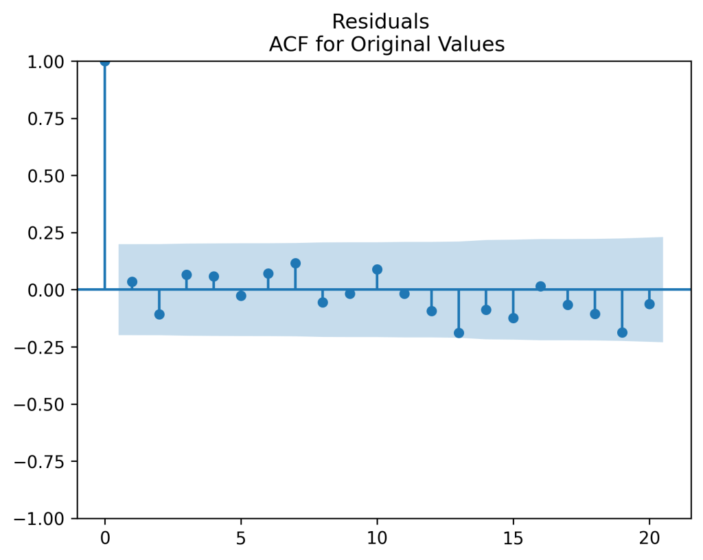
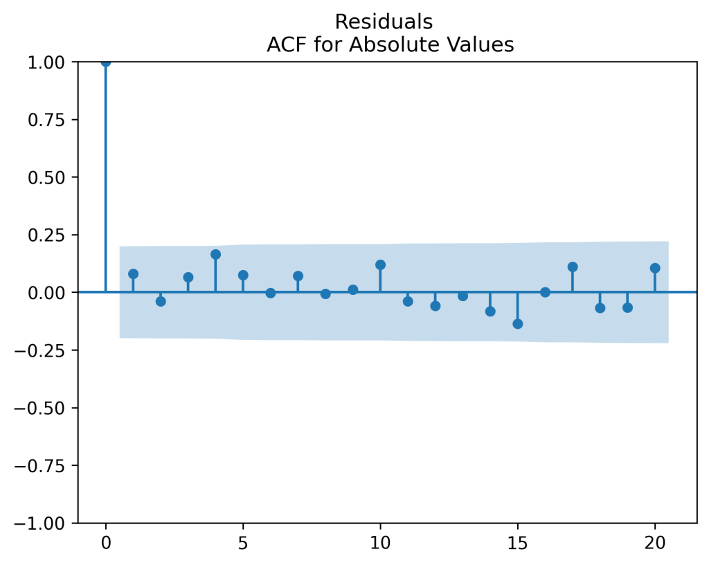
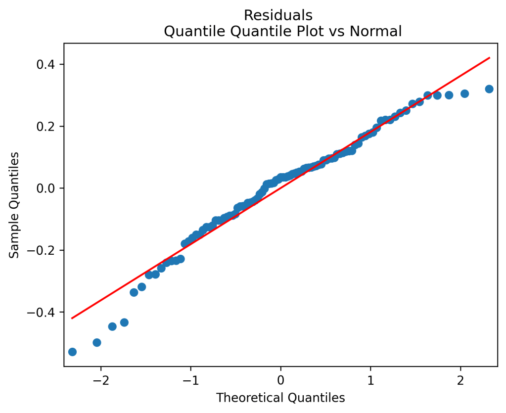
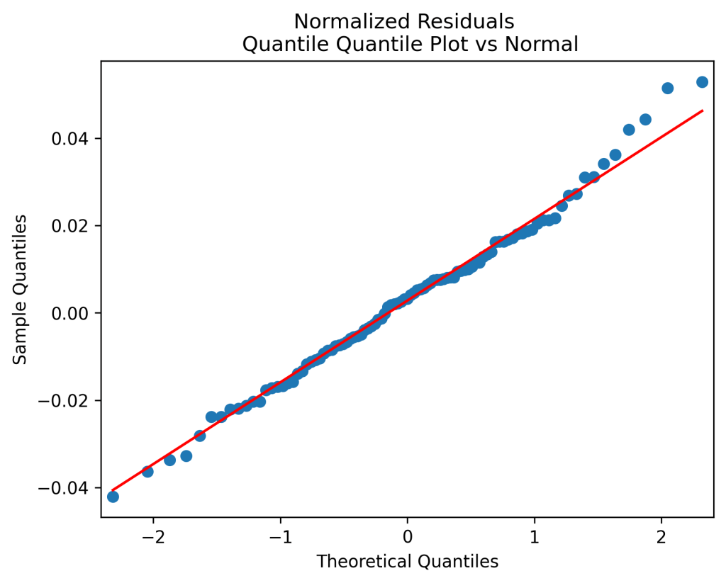
Original model fit: We get innovations which are IID but not quite Gaussian. See plots below. Also, the Shapiro-Wilk and Jarque-Bera tests give us  p = 1.6\%,\quad p = 3.5\%. The Student test for  b = 1 gives us  p 0/3\% so the model is not a random walk, but rather mean-reverting.

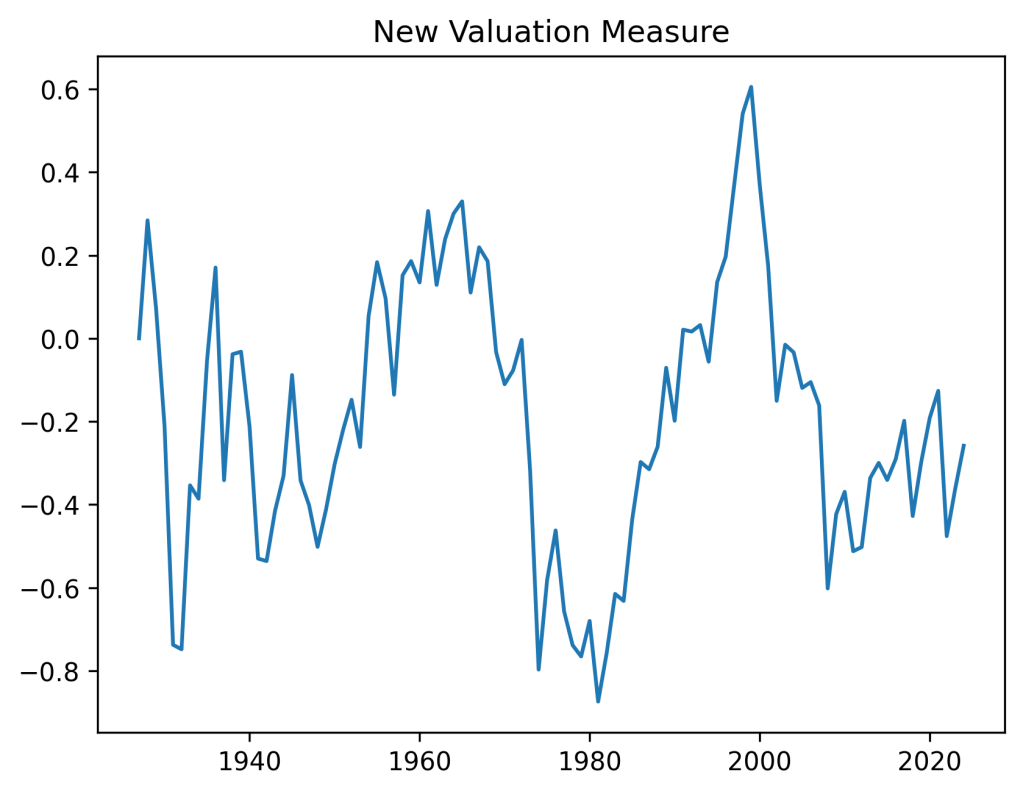
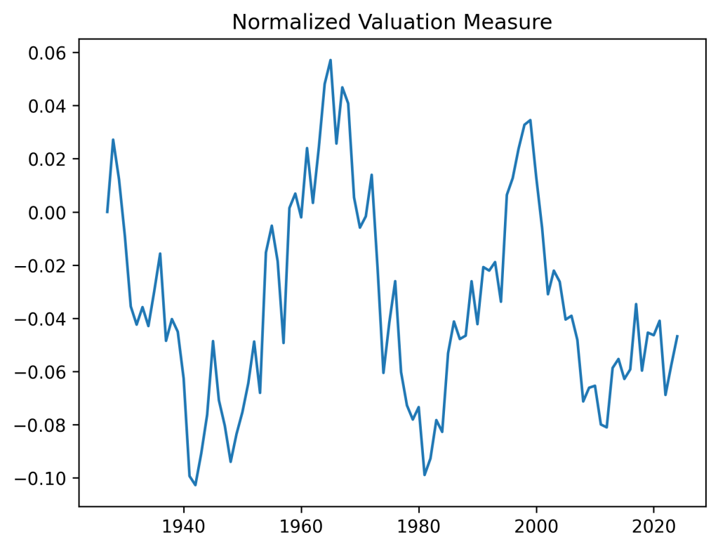
Bubbles and busts: The valuation measure has plot shown below. It is clear that the current valuation measure is well below the historical average. This is in contrast with the classic price-earnings ratio and Shiller CAPE. Both show that the S&P is currently overvalued. However, on the graph below we can see the overvaluation right before the Great Depression, in the 1960s, and at the start of the 21st century (the dotcom bubble). This graph is quite similar to the one in arXiv:1950.04603.

Normalize innovations: Next, let us divide innovations  Z(t) by annual volatility  V(t) computed by Angel Piotrowski. The result is better: These are independent identically distributed Gaussian. Strange high autocorrelation at lag four does not change the suggestions that the innovations indeed can be modeled as IID. Shapiro-Wilk and Jarque-Bera normality tests are  p = 81\%, 71\%.

In other words, it is reasonable to model  H(t) - h = b(H(t-1) - h) + V(t)\delta(t) where  \delta(t) \sim \mathcal N(0, \sigma^2).

Normalize regression, not residuals: Alternatively, we can divide implied dividend yield by volatility and perform this autoregression for the new terms: Consider  \Delta(t) := \Delta(t)/V(t) and repeat the analysis. See the plot of the valuation measure below. It looks very similar to the one above.

Again, the Student T-test gives us  p = 1.1\% for  b = 1. Next, the Shapiro-Wilk and Jarque-Bera tests for new innovations  Z(t) give us  p = 75\%, p = 62\%. The autocorrelation function plots for  Z(t) and for  |Z(t)| show it is reasonable to model these as independent identically distributed, and look very similarly to the above plots for  \delta(t) instead of  Z(t). Further, the quantile-quantile plot for  Z(t) looks very similarly to the one for  \delta(t).

The  R^2 = 8.9\% for original regression and  R^2 = 6.8\% for new regression. We leave it to the reader which one to use. But we intend to use the original regression for future financial simulator.

Update: We used the new regression in the financial simulator. We use the version without the volatility factor, which after division becomes the intercept of the ordinary least squares new regression. This makes the innovations multiplied by this volatility, but does not introduce any new factors in this model. We only compare total returns and earnings growth.

Published by


Responses

  1. Combined Simulator of Annual S&P Returns vs Volatility + (maybe) Earnings Yield – My Finance

    […] research will include Shiller CAPE (with various averaging windows), the new valuation measure (also adapted for various averaging windows), and bond […]

    Like

  2. Annual simulator with volatility and the new valuation measure of S&P 500 – My Finance

    […] the research in the blog post and using the Python code from my GitHub repository, I made a simulator of the Standard & Poor […]

    Like

  3. Using both new valuation measure and CAPE – My Finance

    […] this post, we regress annual total real returns of S&P 500 vs both new valuation measure and the cyclically adjusted price-earnings ratio (Shiller CAPE) with averaging window of 5 or 10 […]

    Like

  4. To Do List – My Finance

    […] Previously, we modeled large stock returns (measured by S&P) using annual volatility and the new valuation measure. We also used bond spreads but not rates, including them in our model. Our next actions […]

    Like

  5. Does the new valuation measure need volatility? – My Finance

    […] do comparison of the new valuation model with or without volatility, for nominal or real version of earnings. We discuss which has the best […]

    Like

  6. Valuation Measure and Long-Short Spread in the Simulator – My Finance

    […] price-earnings ratio (CAPE), for which he got a Nobel Prize in Economics. We discussed it here and here and […]

    Like

  7. Simulator Final Update – My Finance

    […] updated the online simulator to include the bubble measure involving earnings growth, and the long-short spread. The previous version included only the BAA […]

    Like

Leave a reply to To Do List – My Finance Cancel reply