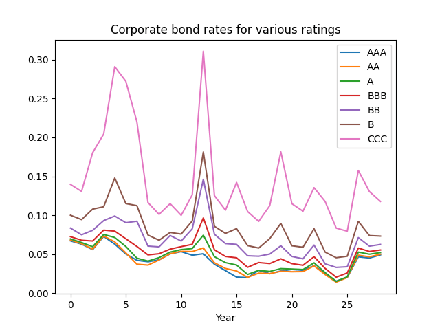
Bank of America Corporate Bonds: Annual Rates

Here we use annual volatility to model bond rates: annual, end-of-year 1996-2024. We take Bank of America bond portfolios with the following seven rates: AAA, AA, A, BBB (investment-grade) and BB, B, CCC (junk, high-yield). Data and code are available on GitHub/asarantsev depository Annual-Bank-of-America-Rated-Bond-Data.

First, consider the rate on the last day of years 1996-2024. Below is the graph of them.

Let $R(t)$ be this rate at end of year $t.$ Model as an autoregression:

$R(t) - R(t-1) = a + bR(t-1) + \delta(t).$

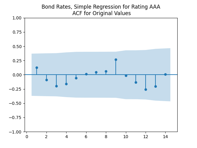
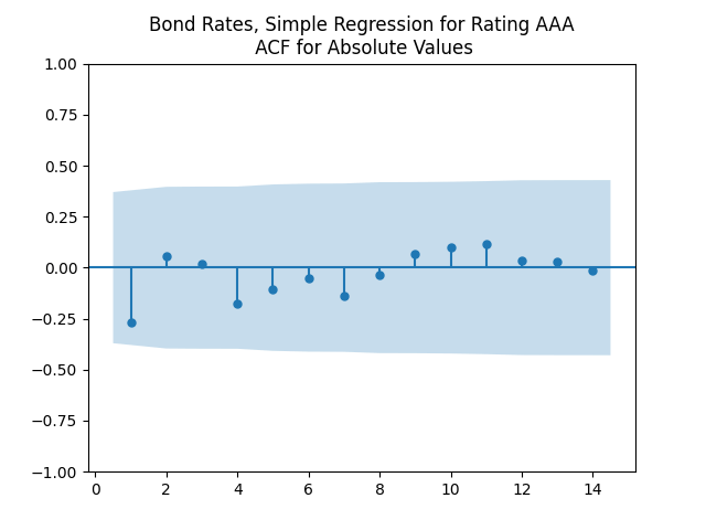
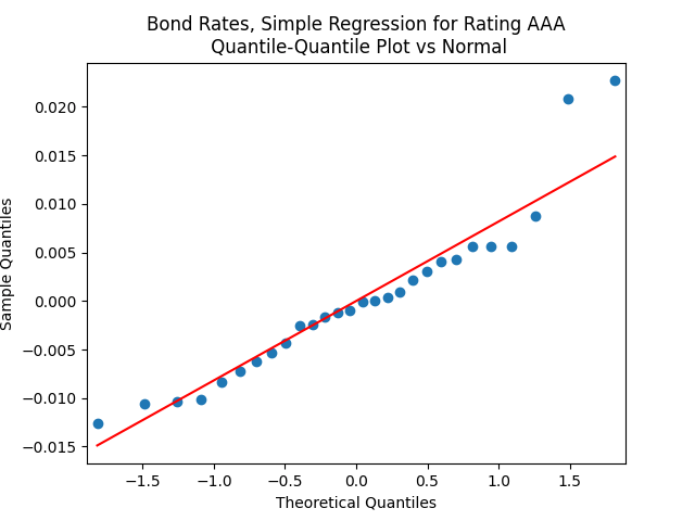
And the results are available in the table below. The last three columns are: Autocorrelation function for innovations, sum of absolute values of the first 5 lags (ACFO); same but for absolute values of innovations (ACFA); Pearson test for $b = 0.$

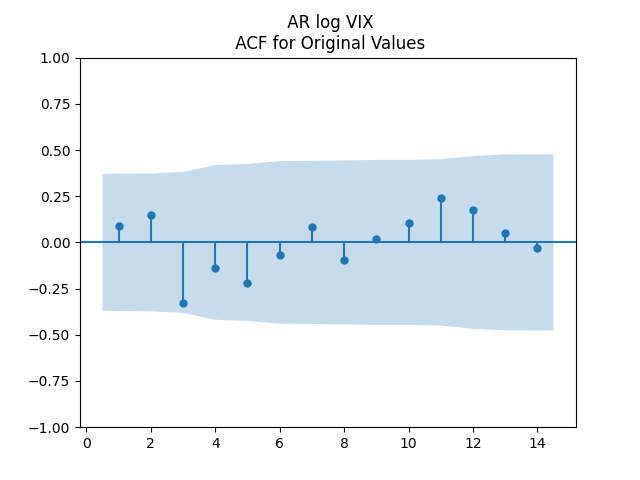
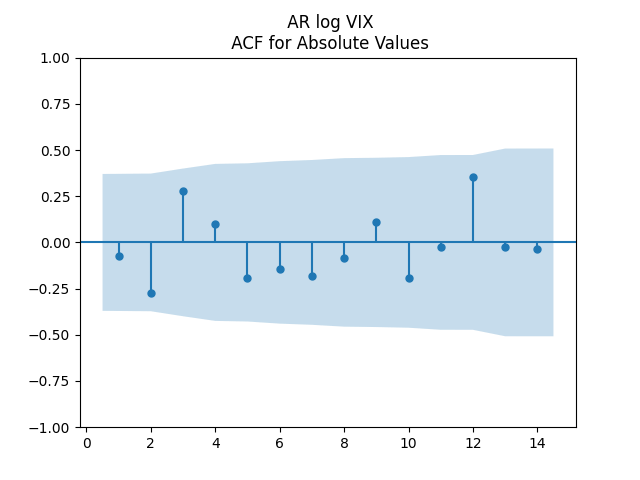
The autocorrelation function (ACF) plots for $\delta(t)$ and for $|\delta(t)|$ shows that this is well explained by independent identically distributed random variables (white noise). But these are not necessarily normal, judging by the Shapiro-Wilk and Jarque-Bera normality tests. Especially for junk-rated bonds (BB, B, CCC) but also sometimes for investment-grade bonds. The random walk hypothesis could be rejected (using low $p$ values) for all rates (even AAA is just barely above $5\%$ ). See also the plots below. We present only the plots for AAA, other ratings are similar. One can generate these graphs by running the code from the GitHub repository mentioned above.

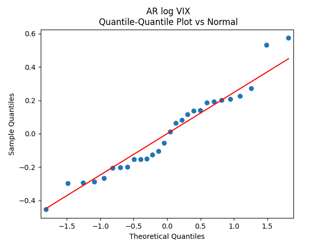
As usual, we can improve fit and make innovations Gaussian by dividing them by annual volatility. Now we take average annual VIX instead of monthly. This parallels research by Angel Piotrowski mentioned in previous posts. But she computed annual realized volatility, and I use averaged VIX (implied volatility). Let us first fit the log Heston model for VIX 1996-2024:

$\ln V(t) = \alpha + \beta \ln V(t-1) + W(t).$

Here, $\alpha = 1.41$ and $\beta = 1 - 0.475.$ Next, $R^2 = 23.5\%$ and $p = 0.9\%$ for Student $t$ test for $\beta = 1.$ The standard deviation for $W(t)$ is $0.247.$ The normality tests for innovations $W(t)$ give us $p = 27.5\%$ for Shapiro-Wilk and $p = 60.8\%$ for Jarque-Bera. The plots for ACF of $W(t)$ and for $|W(t)|$ show independent identically distributed. See below. Thus the log volatility is indeed modeled by the autoregression of order 1, statistically significantly mean-reverting, with Gaussian innovations. This is similar to Angel Piotrowski’s research.

Consider the autoregression with normalization of innovations $\delta(t)$ by dividing them by volatility $V(t).$ We have then

$R(t) = a + bR(t-1) + V(t)\,\varepsilon(t).$

Divide by VIX and then get an ordinary least squares regression with residuals $\varepsilon(t)$ without intercepts. Let us add intercepts:

$R(t) = a + bR(t-1) + cV(t) + V(t)\,\varepsilon(t).$

Results are available below in the table: Coefficients and analysis of innovations $\varepsilon(t).$

All correlation between $W(t)$ and $\varepsilon(t)$ are not statistically significant. For investment-grade ratings, we have $p$ higher than 5% for all coefficients. But for junk ratings, $p < 5\%$ for $b = 0.$ And for the two bottom ratings, $p < 5\%$ for $c = 0.$ Next, $R^2$ for linear regression with $cV(t)$ for most ratings is much higher than without it. So we need to include this term.

Thus we see a joint model: For $\beta \in (0, 1)$ and $b \in (-1, 0)$ we get:

$\ln V(t) = \alpha + \beta \ln V(t-1) + W(t)$

$R(t) - R(t-1) = a + bR(t-1) + cV(t) + V(t)\varepsilon(t)$

$(W(t), \varepsilon(t)) \sim \mathcal N_2([0, 0], \Sigma)$ IID

As discussed, we might consider $\Sigma$ to be the diagonal matrix, but might as well make it a complete matrix. This model fits very well. A disadvantage is that we have only ~30 years of data. We do need to normalize innovations of rates by dividing these by VIX. We do need the term $cV(t).$

In our previous research, we proved long-term stability of this bivariate model. This is true not just for Gaussian innovations, but for more general cases, under certain conditions.

We continue this research in the next post, where we model total returns.

Responses

Bank of America rated bonds: Annual Returns – My Finance

February 25, 2025 at 8:59 pm

[…] of research in github.com/asarantsev repository Annual-Bank-of-America-Rated-Bond-Data from my previous post. Consider total returns computed from total wealth process as log change: If these were Treasury […]

LikeLike

Investment-Grade Corporate Bond Returns 1972-2024 – My Finance

February 27, 2025 at 6:59 pm

[…] the two previous blog posts, we considered rates and returns for Bank of America-rated corporate bond portfolios, with ratings AAA, AA, A, BBB, BB, […]

LikeLike

Annual Corporate Bank of America Rates – My Finance

April 10, 2025 at 10:27 am

[…] from the previous post, which in turn continues the two posts of annual Bank of America-rated bond rates and returns. We fit the 1996-2024 data for corporate bond returns and […]

LikeLike

Rate	$b$	$a$	Stdev of residuals	Skew	Kurtosis	Shapiro-Wilk $p$	Jarque-Bera $p$	ACFO	ACFA	Pearson Test $p$
AAA	-0.21	0.0081	0.008	0.994	1.241	0.029	0.041	0.629	0.627	0.051
AA	-0.23	0.0087	0.009	0.747	0.842	0.108	0.18	0.716	0.918	0.049
A	-0.26	0.011	0.01	0.571	0.53	0.138	0.397	0.48	0.744	0.043
BBB	-0.33	0.017	0.012	0.799	1.671	0.09	0.044	0.262	0.699	0.025
BB	-0.46	0.031	0.02	1.479	3.951	0.007	<0.001	0.482	0.814	0.009
B	-0.57	0.048	0.026	1.612	3.629	0.003	<0.001	0.366	0.727	0.003
CCC	-0.57	0.082	0.055	1.338	2.051	0.007	0.001	0.576	0.626	0.004

Rate	$a$	$b$	$10000*c$	Stdev	Skew	Kurt	S-W	J-B	ACFO	ACFA
AAA	0.01	-0.14	-2.41	0.00037	0.774	0.664	22%	19%	0.352	0.816
AA	0.0099	-0.116	-2.78	0.0004	0.67	0.807	43%	24%	0.402	0.924
A	0.0087	-0.157	-1.06	0.00044	0.342	0.2	93%	74%	0.395	0.963
BBB	0.0099	-0.279	-2.1	0.00051	0.039	-0.4	96%	91%	0.405	0.779
BB	0.015	-0.539	10.0	0.00076	0.303	-0.21	88%	79%	0.656	0.594
B	0.0235	-0.77	20.3	0.00096	0.35	-0.126	46%	74%	0.576	0.722
CCC	0.0217	-0.73	41.5	0.00198	0.58	0.25	36%	44%	0.817	0.948

Bank of America Corporate Bonds: Annual Rates

Share this:

Responses

Leave a reply to Investment-Grade Corporate Bond Returns 1972-2024 – My Finance Cancel reply