My Finance

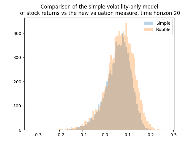
Continuing the previous blog, I wrote combined simulator for Standard & Poor 500 annual total returns with two options:

• Annual realized volatility only, computed by my undergraduate student Angel Piotrowski
• Volatility + earnings yield, earnings is averaged over the last few years. Averaging window ranges from 1 to 10 years.

I do not think combining these simulators in one Python code file works well. Indeed, when you add more and more features and options, it becomes harder to manage them. Better to create multiple Python files for each option. In the main Python file we can import all other files and organize input of options. If a user chooses an option, the main Python file should redirect to another Python file which does computation for this chosen option.

But I uploaded the Python code to GitHub/asarantsev repository earnings-yield-annual-simulator.

Setting: Withdrawals 40 per year: 4% of the initial capital (inflation-adjusted). Time horizon is long: 30 years. As before for cyclically adjusted price-earning ratio: CAPE, we do not allow the choice of initial conditions: We pick them to coincide with current (as of December 2024) market conditions.

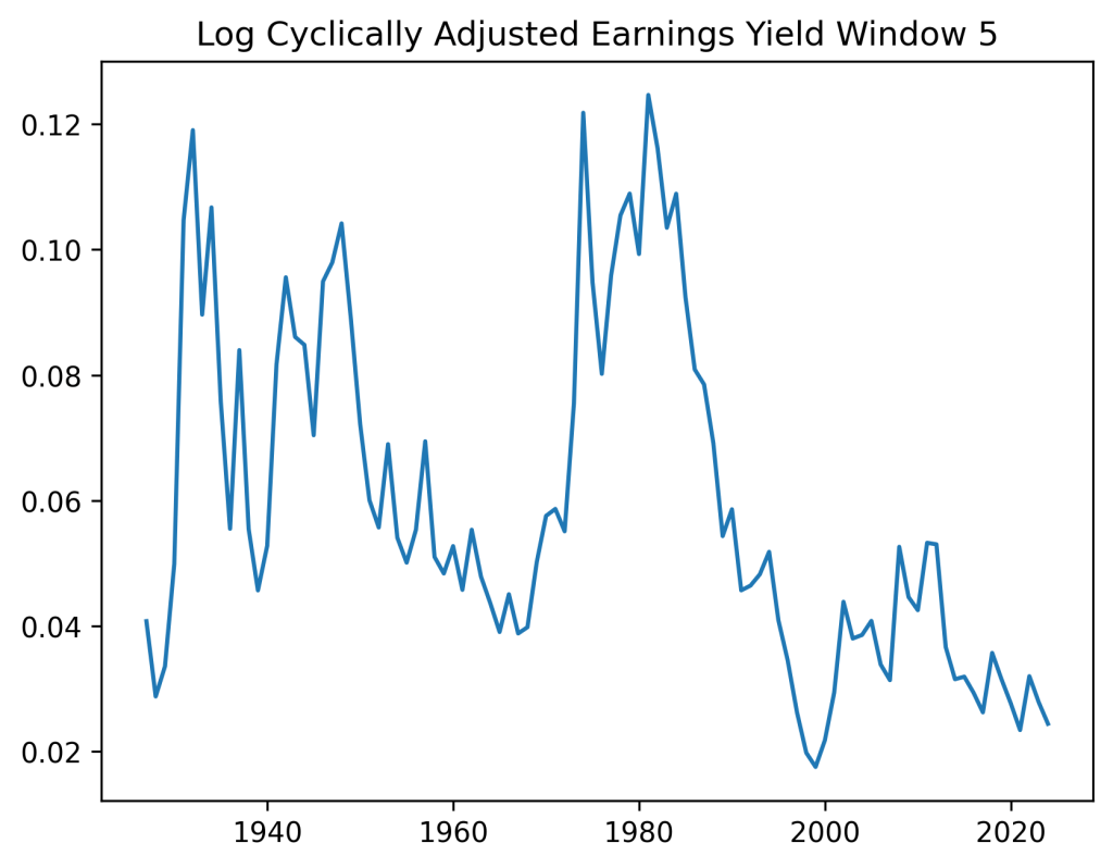
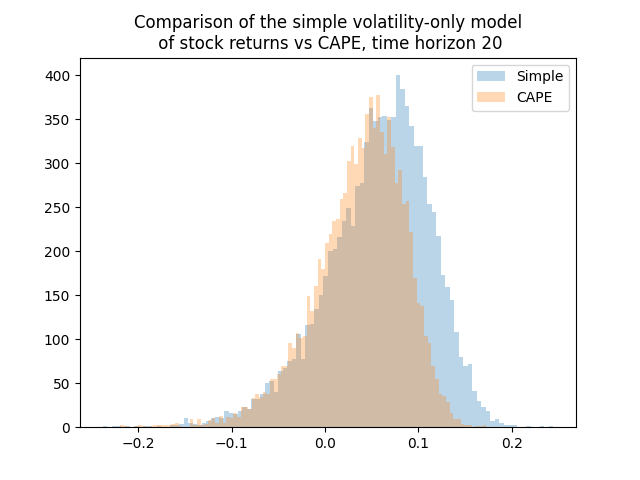
Results: Cyclically adjusted earnings yield currently is much lower than historical average. This is equivalent to CAPE being much higher than historical average. This implies lower future returns than historically, and higher ruin probability.

We can also see high variance of final wealth: Greatly skewed to the right. A few top simulations have huge wealth. This might be due to including earnings yield, instead of its logarithm. Then the time series model (in continuous time this would be a stochastic differential equation) for total returns has an exponentially increasing drift.

Modification: Let us change the earnings yield factor to its logarithm in regressions for price and total returns. Then the variance of final wealth is much less, and less skewed to the right. That is, unrealistic very high wealth outliers are much less likely. See below the graph. But returns are still much lower than for historically average earnings yield. We still refer to the same GitHub/asarantsev repository earnings-yield-annual-simulator.

We combine two models: S&P total returns vs volatility only or vs volatility and earnings yield. See the data and code in https://github.com/asarantsev/earnings-yield-annual-simulator

This research continues blog posts on modeling returns vs earnings yield and volatility and returns vs only volatility. But previous Python code combines fitting of this model and simulation. Here, we removed plots (quantile-quantile and autocorrelation function for residuals) and analysis of skewness, kurtosis, etc. We only keep fitting regression code necessary for actual simulations. Also, we combine these two options (with or without earnings yield) so a person can make a choice. We also present a choice between simulating innovations using Gaussian multivariate distribution or kernel density estimation.

We also change the models slightly: Previously, we normalized returns and earnings growth by dividing them by annual volatility Here, we instead model these as regression

Future research will include Shiller CAPE (with various averaging windows), the new valuation measure (also adapted for various averaging windows), and bond spreads.

Background: I continue the previous post of joint work with my undergraduate student Angel Piotrowski. Consider my work arXiv:1905.04603. We wrote about this in yet another post. In a GitHub/asarantsev repository we updated our code and data.

Let be the 10-year trailing averaged annual real earnings. Let be the log growth terms. We compute these for Also, let be total real returns for the same years. Then is implied dividend yield; we assume is its long-term average. We model the valuation measure as an autoregression of order 1:

where innovations are independent identically distributed, with mean zero.

As discussed before, the difference between our research and arXiv:1905.04603 is that we take December CPI data instead of January to compute inflation, and end-of-year S&P index data instead of average January close level. Also, we consider 10-year instead of 5-year trailing window for real earnings.

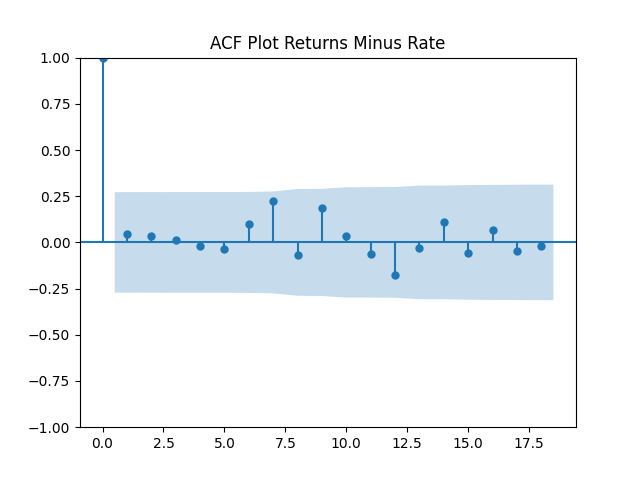
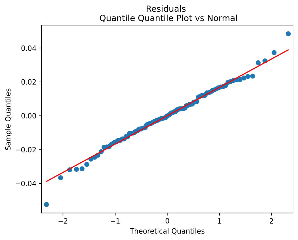
Original model fit: We get innovations which are IID but not quite Gaussian. See plots below. Also, the Shapiro-Wilk and Jarque-Bera tests give us The Student test for gives us so the model is not a random walk, but rather mean-reverting.

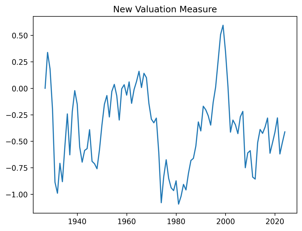
Bubbles and busts: The valuation measure has plot shown below. It is clear that the current valuation measure is well below the historical average. This is in contrast with the classic price-earnings ratio and Shiller CAPE. Both show that the S&P is currently overvalued. However, on the graph below we can see the overvaluation right before the Great Depression, in the 1960s, and at the start of the 21st century (the dotcom bubble). This graph is quite similar to the one in arXiv:1950.04603.

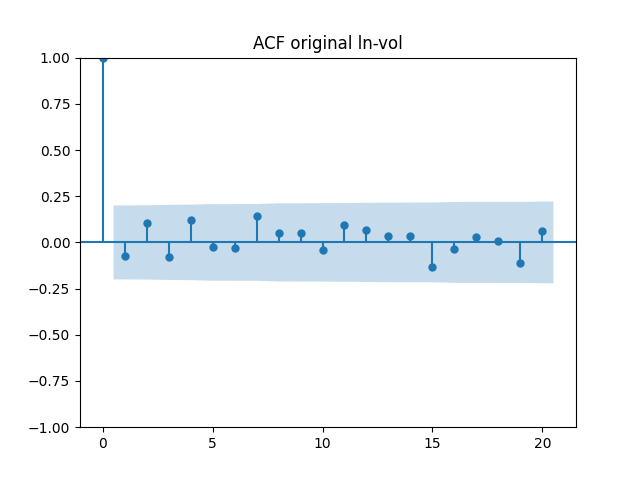
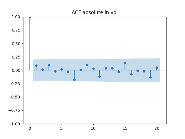
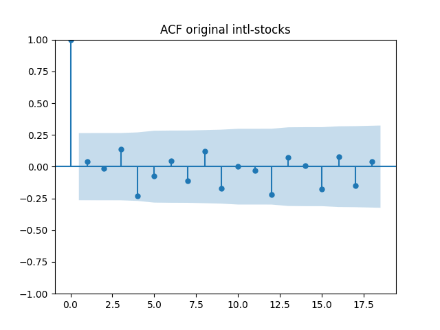
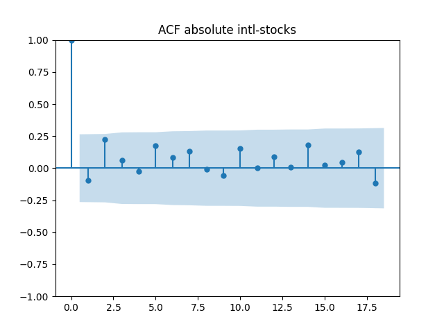
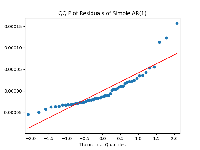
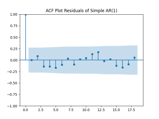
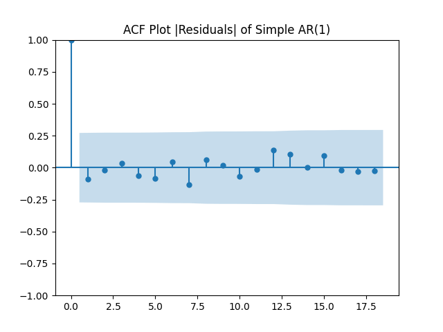
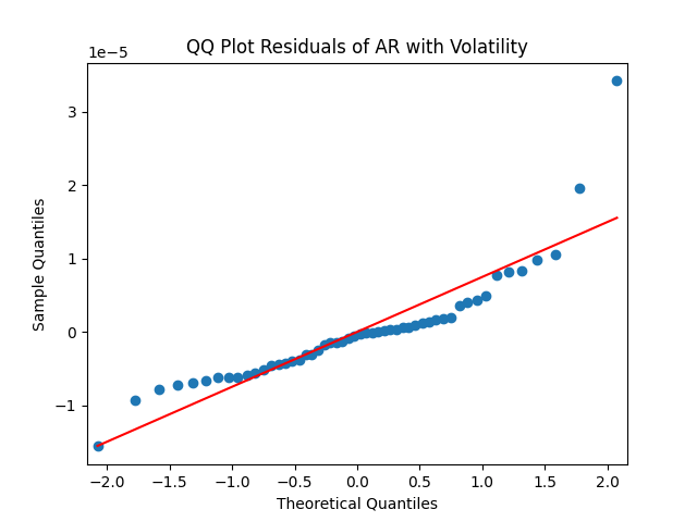
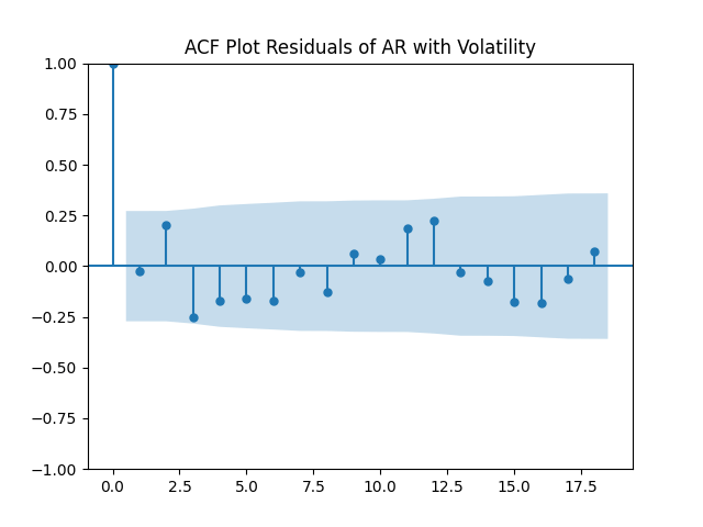
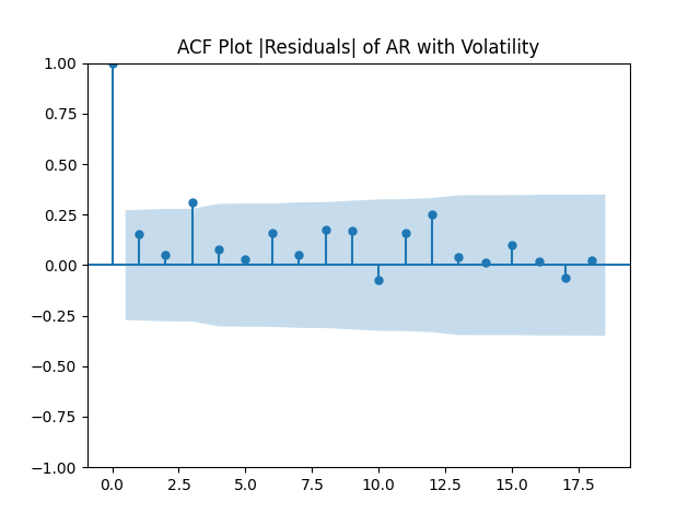
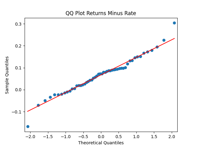
Normalize innovations: Next, let us divide innovations by annual volatility computed by Angel Piotrowski. The result is better: These are independent identically distributed Gaussian. Strange high autocorrelation at lag four does not change the suggestions that the innovations indeed can be modeled as IID. Shapiro-Wilk and Jarque-Bera normality tests are

In other words, it is reasonable to model where

Normalize regression, not residuals: Alternatively, we can divide implied dividend yield by volatility and perform this autoregression for the new terms: Consider and repeat the analysis. See the plot of the valuation measure below. It looks very similar to the one above.

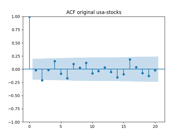
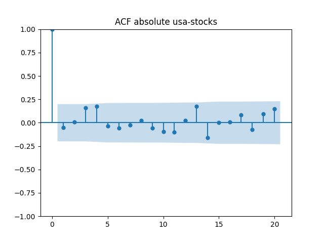
Again, the Student T-test gives us for Next, the Shapiro-Wilk and Jarque-Bera tests for new innovations give us The autocorrelation function plots for and for show it is reasonable to model these as independent identically distributed, and look very similarly to the above plots for instead of Further, the quantile-quantile plot for looks very similarly to the one for

The for original regression and for new regression. We leave it to the reader which one to use. But we intend to use the original regression for future financial simulator.

Update: We used the new regression in the financial simulator. We use the version without the volatility factor, which after division becomes the intercept of the ordinary least squares new regression. This makes the innovations multiplied by this volatility, but does not introduce any new factors in this model. We only compare total returns and earnings growth.

This is a big post (the biggest on blog so far) which extends our previous posts:

• Four bond rates from 1927
• S&P 500 Returns using Earnings Yield and Volatility
• Dividing annual earning growth by volatility makes them Gaussian white noise
• Vector autoregression with volatility for two spreads
• Growth/Volatility vs Spreads
• Stock Returns vs Earnings Yield and Two Spreads
• Make S&P Returns IID Gaussian
• Does dividing by volatility improve fit for bond spread?

The data is available on my personal web page. The code is available on my GitHub/asarantsev repository 3spreads-1yearnyield-returns which contains 3 Python code files corresponding to 3 parts of this post:

• PART 1. Modeling bond spreads BAA-AAA, AAA-Long, Long-Short as vector autoregression
• PART 2. Modeling earnings growth using these bond spreads as regression factors
• PART 3. Modeling S&P returns using 1-year earnings yield and these bond spreads as regression factors

PART 1: Modeling bond spreads BAA-AAA, AAA-Long, Long-Short using vector autoregression of order 1, with innovations normalized by annual volatility. This model fits well and is stable in the long run, with IID but not quite Gaussian innovations.

Data: We consider four bond rates, average daily December data 1927-2024, at end of year t:

1. Long stands for 10-year Treasury rate (1963-now), long-term government securities (1927-1962)
2. Short stands for 3-month Treasury rate (1934-properly extended to earlier data), and short-term (3- and 6-months) government securities (1927-1933)
3. BAA is Moody’s rates for portfolios of investment-grade corporate bonds with BAA ratings (1927-2024)
4. AAA is Moody’s rates for portfolios of investment-grade corporate bonds with AAA ratings (1927-2024)
5. Annual realized volatility of Standard & Poor 90/500 (1928-2024) daily log returns for year

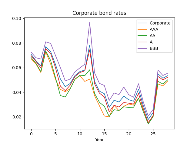
See the time graph of interest rates below. This continues research from the previous blog post.

Next, we take three bond spreads: BAA-AAA, AAA-Long, Long-Short. See the time graph below.

Model: Consider the vector S(t) of three bond spreads. We model it as where and is a 3\times 3 matrix, and is a sequence of independent identically distributed (IID) trivariate random vectors with mean zero. This is an extension of the same model for two spreads: BAA-AAA and AAA-Long, which, in turn, continues this research.

As usual, we also have log Heston model for the volatility: where are IID with mean zero. We already fit it in the previous post, so we do not discuss it here.

We fit this multivariate model for by each of three scalar equations. We divide this equation by the volatility and then use ordinary least squares method. Then we test each of the three components of the innovation series for IID Gaussian using the usual procedure:

1. Empirical skewness and kurtosis (both = 0 for Gaussian)
2. Shapiro-Wilk and Jarque-Bera normality tests p-values
3. L1 norm for the autocorrelation function for lags 1, \ldots, 5, of and
4. Autocorrelation function plots for and for
5. The quantile-quantile plot of versus the normal distribution

Results for coefficients: We have the following point estimates:

The Student T-test gives us only for diagonal values of B, its third row, and c. It is important to verify that eigenvalues of B are strictly less than 1. Then the time series model above is stable and ergodic in the long-run, see my manuscript arXiv:2411.03699: Zero-Coupon Treasury Rates and Returns using the Volatility Index with Jihyun Park. It has a unique stationary distribution, see this work. But this is left for further research.

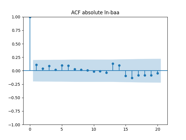
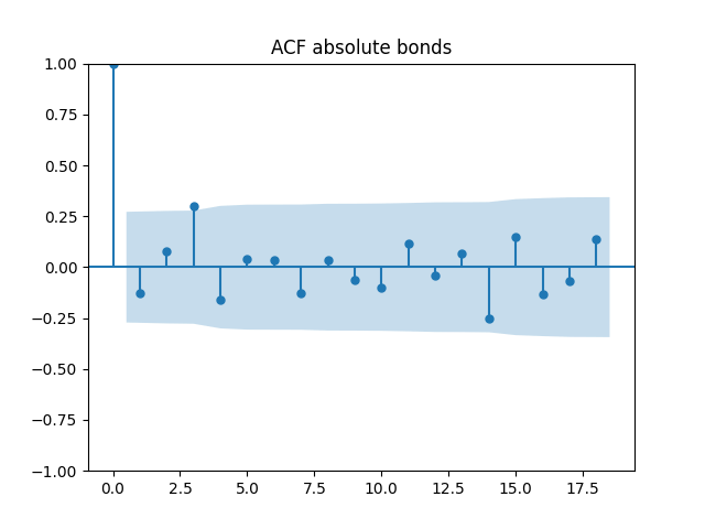
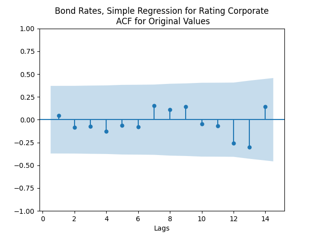
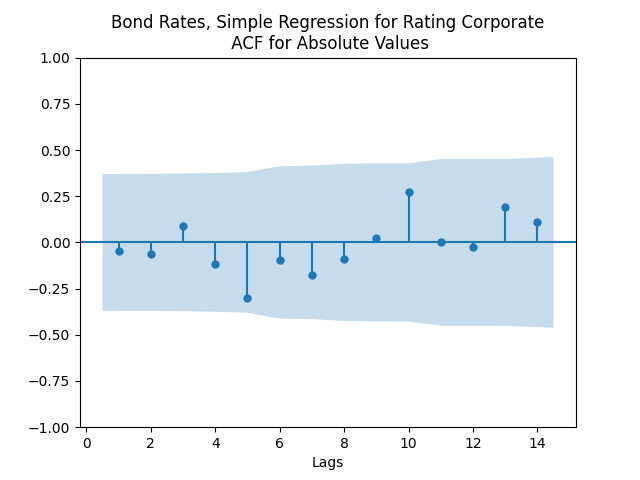
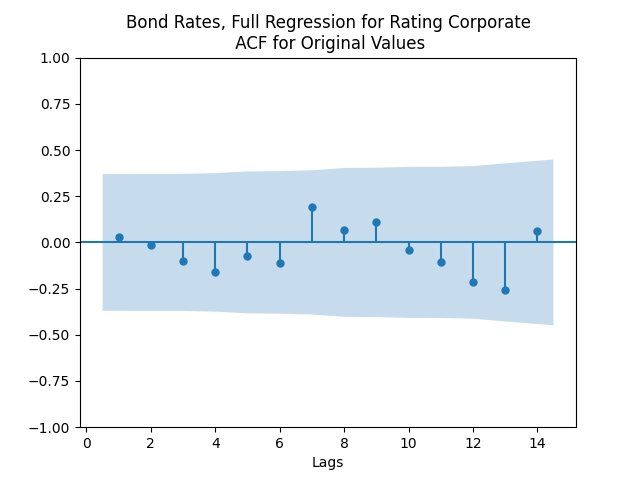
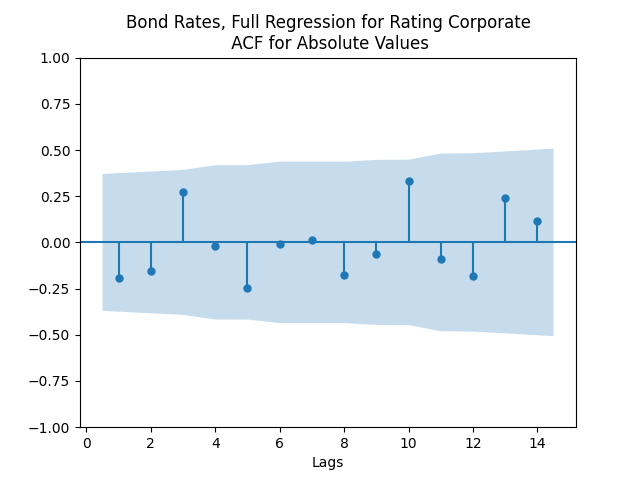
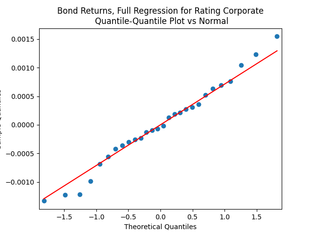
Results for innovations: They can be modeled as IID. The plots are shown below for each of the three series of residuals. First, Moody means BAA-AAA spread. Although we have strange ACF for lag 1 for absolute values, overall the plots are consistent with IID.

Second, Risk means AAA-Long spread. Here, we have a very good fit for IID.

Finally, Term means Long-Short spread. We also have this strange autocorrelation at lag 1 for absolute values.

Unfortunately, we did not test the cross-correlation functions and plots, similarly to this post. We failed to do this because of lack of time, and because Python lacks a built-in function for such plots, unless you use a simple vector autoregression without volatility. But previous modeling of closely related modeling suggests that these cross-correlation functions will not be significantly different from zero.

The values of L1 norm for the first five lags of ACF from each of the 3 spreads above are:

Spread	BAA-AAA	AAA-Long	Long-Short
Original	0.445	0.539	0.328
Absolute	0.515	0.606	0.431

Recall the critical values for the L1 version of the Ljung-Box white noise test. Comparing them with our values here, we confirm we fail to reject the white noise hypothesis.

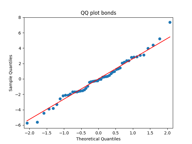
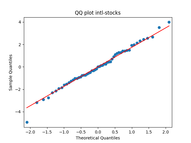
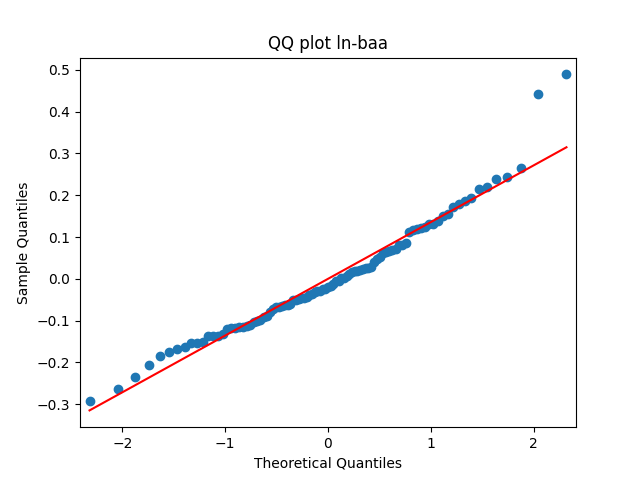
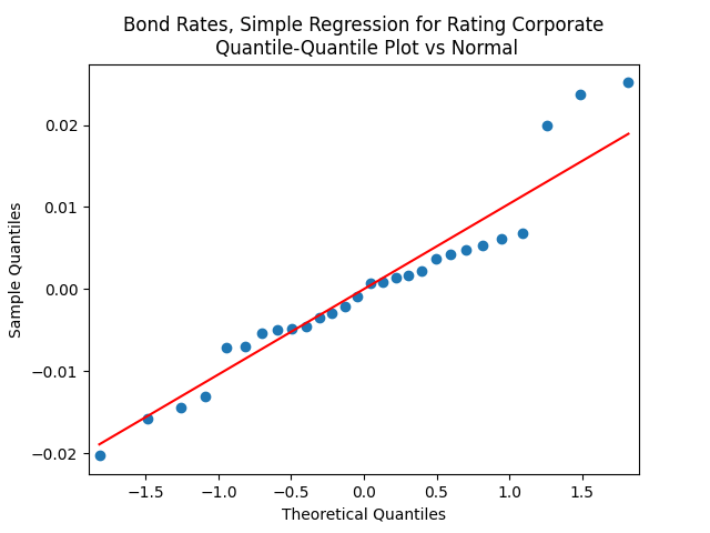
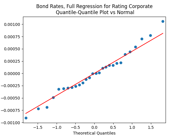
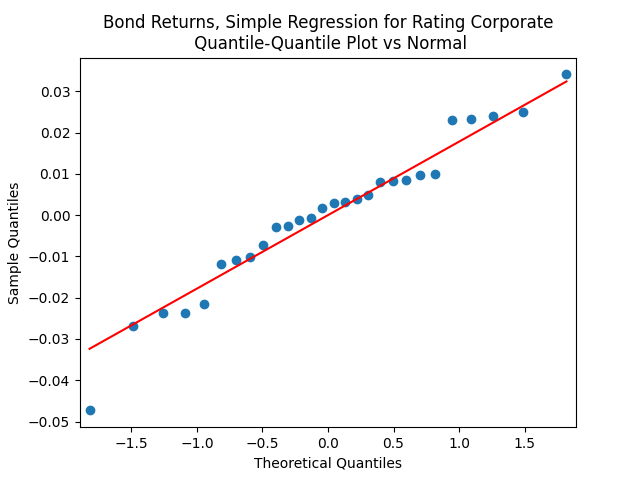
Innovations are not Gaussian, but quite close. See the quantile-quantile plots. Also, below are normality statistics.

Spread	BAA-AAA	AAA-Long	Long-Short
Skewness	0.557	0.683	-0.097
Kurtosis	0.594	0.635	1.338
Shapiro-Wilk p	1.3%	0.6%	4.3%
Jarque-Bera p	4.0%	1.0%	2.5%

PART 2: Modeling earnings growth (nominal/real) using these 3 bond spreads as regression factors, with innovations normalized by annual volatility. This model fits well, with IID but not quite Gaussian innovations.

Data: In addition to the data from PART 1, we have annual data 1927-2024: Denote December data for year t by Further, let be annual earnings 1928-2024 for S&P 90/500. These can be real (inflation-adjusted) or nominal (not inflation-adjusted). Then is log earnings growth from year to year

Model 1: We modeled it earlier as IID after dividing by volatility: But here, we model these normalized growth terms using regression versus these three spreads: Here, is a constant, is a vector, and are IID with mean zero.

Model 2: Alternatively, we can model Here we normalize residuals by volatility. Here, again are IID with mean zero, is a vector and are scalars. This is different from the first model, where we normalize growth terms but not spreads. We fit this model after dividing this equation by

Methodology: We analyze residuals for IID Gaussian, as in PART 1, using the five-point program.

Results: All four regressions (Models 1 and 2, nominal and real) have IID residuals (judging by ACF values and plots), which are close to normal (judging by the quantile-quantile plots) but unfortunately not quite normal (judging by normality tests, skewness, and kurtosis). See plots below for Model 1 = normalized spreads, Model 2 = original spreads.

For Model 1, the only significant coefficient with is for Long-Short, judging by Student T-test. For Model 2, this is AAA-Long. All other .

For Model 1, (nominal) and (real). For Model 2, for both nominal and real.

PART 3: We model S&P annual returns (total/price, nominal/real) normalized by S&P volatility using linear regression upon three spreads: BAA-AAA, AAA-Long, Long-Short, and earnings yield. Residuals are IID Gaussian.

Data: We have 1927-2024 S&P 90/500 index data:

• end of year (last trading day close) level, 1927-2024;
• annual dividends and earnings, 1928-2024;
• annual realized volatility (standard deviation of log level daily changes), 1928-2024;
• Consumer Price Index December data, 1927-2024.

This allows us to compute four versions of index returns We allow for following options: price (excluding dividends) and total (including dividends); nominal (not adjusted for inflation) and total (adjusted for inflation). Also, we can compute earnings yield This is the ratio of annual earnings this year to end-of-year index level. See the graph below. We have a big drop in 2008 since earnings drop there much faster than index.

As above, we also have four December daily average rates: BAA, AAA, Long and Short, for 1927-2024. This allows us to compute these three spreads. We studied these spreads and used these to model earnings yield before. Denote their vector as

Model 1: Consider the linear regression Here, are IID with mean zero. Next, are scalars and

Model 2: Remove earnings yield from this regression and fit it again:

Model 3: Remove all spreads: make Then

Model 0: Remove both spreads and earnings yield: Then we get Compare with this post.

Methodology: Divide these equations by volatility and fit regressions using ordinary least squares. Use the 5-point program from Part 1 of this post to analyze residuals.

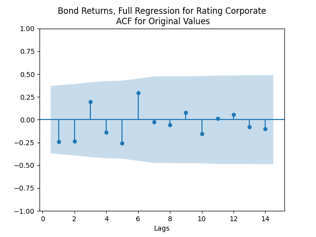
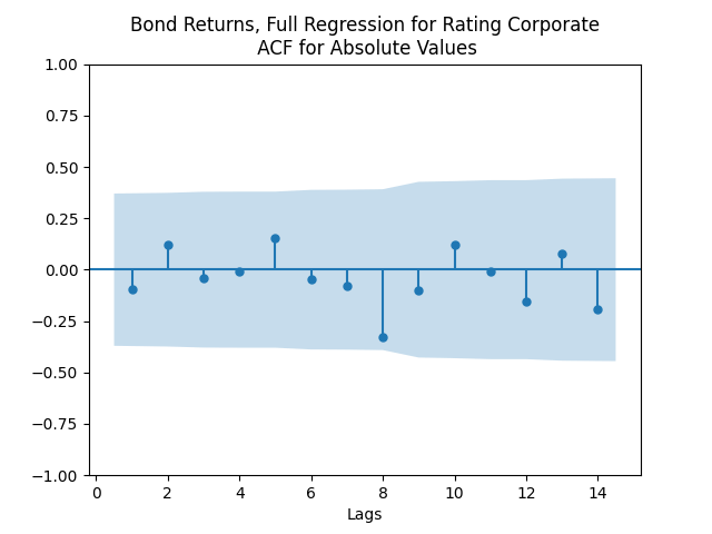
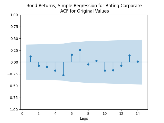
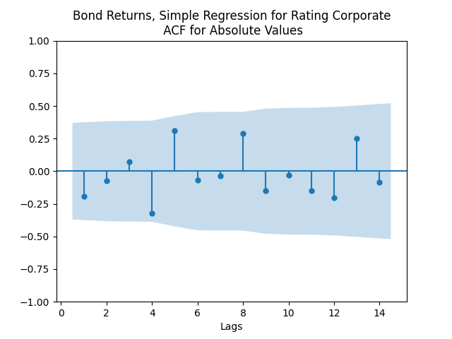
Results: Autocorrelation Function (ACF) plots for and for confirm IID. However, we still have this strange high value in lag 4, similar to the previous blog post. Computation of L1 norm for first 5 lags of ACF for and for also confirm IID.

Also, Shapiro-Wilk and Jarque-Bera tests show normality. All

Coefficients for spreads are not significantly different from zero, judging by the Student T-test, for each of four types of returns. But removing these coefficients greatly reduces We also fail to reject Judging by the value for Student T-test, these spreads are BAA-AAA, AAA-Long, Long-Short in decreasing order of importance. I think it is best to use the full version of this regression.

Conclusion: The overall model for the following quantities:

• end-of-year bond spreads BAA-AAA, AAA-Long, Long-Short:
• annual S&P 500 earnings
• end-of-year S&P 500 level
• annual realized S&P 500 volatility
• annual total S&P 500 returns

Here are independent identically distributed with mean zero, but not Gaussian.

This research is continued in the post where we consider trailing averaged annual earnings, with a window up to 10 years.

Model description: Continuing research from the previous post on earnings growth and bond spreads, consider the annual December data 1927-2024. We have Standard & Poor returns in four versions:

• total returns (including dividends) vs price returns (excluding dividends);
• nominal returns (not inflation-adjusted) vs real returns (inflation-adjusted).

We have the following three factors, known at end of year

• Earnings Yield: annual earnings / end-of-year price
• Bond spread BAA-AAA (both are rates by Moody’s)
• Bond spread BAA-10YTR (Moody’s BAA rate minus 10-year Treasury rate)

Also, we add annual realized volatility which we add both additively to the linear regression, as a factor, and multiplicatively, to the innovations (residuals). We have the following model:

Summary of results: Instead of giving large tables, we simply provide a short summary and refer an interested reader to the Python code.

• Regression residuals pass Shapiro-Wilk and Jarque-Bera normality test with flying colors. This matches quantile-quantile plots versus the Gaussian distribution.
• The autocorrelation function plots for and for show that white noise conjecture is reasonable. Although, similarly to this post, we have strange large value at lag 4.
• Applying L1 norm for the autocorrelation function and comparing with this simulation, we get values which lie between 0.4 and 0.5 for and between 0.6 and 0.7 for , which are within the 99% interval. Thus we fail to reject the white noise hypothesis.
• Regression factors have large p-values according to the Student T-test. Thus we fail to reject the hypothesis that or or We did not test the joint hypothesis when all these three parameters are zero. But we reject because
• Point estimates in all four cases are

A modification: Instead of earnings yield (which is always positive) take its logarithm: Results are almost the same as described above. Although for nominal total returns the L1 norm for is 0.706.

See the code and data at https://github.com/asarantsev/growth-spread

This is Monte Carlo simulation to find critical values of the L1 version of the Ljung-Box test. I was too lazy to look for the official L2 norm for ACF using the classic Ljung-Box test. I simply decided to simulate.

Consider a sample of 100 standard normal random variables

Compute the empirical autocorrelation function with lag which is an empirical correlation of and Do this for Then compute the L1 norm

Do the same for instead of

Finally, compute empirical mean and the empirical centered moments of order

Then the empirical skewness is and the empirical kurtosis is

We create 1 million simulations of this 100 i.i.d. Gaussian variables. We compute values corresponding to 95% and 99% percentiles of simulated data for 100 IID standard normal (a million simulations). We get the following table (skewness is taken with absolute value, disregarding the sign). See https://github.com/asarantsev/4rates

Function	95% percentile	99% percentile
Skewness	0.47	0.63
Excess Kurtosis (normal = 0)	0.76	1.38
L1 norm for ACF (both), 5 lags	0.63	0.76

Added on June 5, 2025: If we make 100 000 simulation of only 50 i.i.d. Gaussian variables (instead of 100, simply changing this number in the code), we have:

Function	95 percentile	99 percentile
Skewness	0.643	0.878
Excess Kurtosis (normal = 0)	0.977	1.859
L1 norm for ACF (5 lags), original	0.882	1.079
L1 norm for ACF (5 lags), absolute	0.877	1.073

We also simulate skew normal variables with skewness parameter 3. Obviously, the true skewness and excess kurtosis will not be equal to zero any more. But we can still take percentiles for the empirical kurtosis and for these L1 norms for ACF, applied to original values of these variables and to absolute values of these variables. We take only 10000 simulations. For sample of size 100/50, we get:

Function	95 percentile	99 percentile
Excess Kurtosis (normal = 0)	1.92/2.08	3.37/3.92
L1 norm for ACF (5 lags), both	0.63/0.87	0.75/1.06

This is done in the file skewsim.py in the same GitHub repository.

See the GiHub repository https://github.com/asarantsev/growth-spread

Continuing research of Ian Anderson, we model by dividing it by annual volatility Here, is annual (nominal or real) earnings of Standard & Poor 500 and its predecessor Standard & Poor 90. We regress it upon BAA-AAA and BAA-10YTR spreads and studied here. We have data 1927-2024 annual. We take spreads for average daily December values. Consider three possible regressions:

• Model 0:
• Model 1:
• Model 2:
• Model 3:

For each regression, we compute both nominal (not inflation-adjusted) and real (inflation-adjusted) earnings growth. Thus we have 6 models. We compute autocorrelation function plots for each and All these look like white noise. Also, we compute 5-lag L1 norm for autocorrelation function for each of these 6 series of residuals and other 6 series of their absolute values. All these 12 numbers are less than 0.6, which is less than the 95% critical value; see Monte Carlo simulations. The following table shows skewness, kurtosis, and the results of Shapiro-Wilk and Jarque-Bera normality tests.

Series	Skewness (Normal 0)	Kurtosis (Normal 0)	Shapiro-Wilk	Jarque-Bera		p-value for Student test
Nominal	0.479	2.158	0.3%	0.0%	7.2%	32% (volatility)
Real	0.459	1.893	0.7%	0.0%	4.9%	24% (volatility)
Nominal	-0.114	2.105	1.3%	0.0%	4%	5.2% (BAA-AAA) and 6.9% (BAA-10YTR)
Real	-0.136	1.861	2.8%	0.1%	5.2%	5.2% (BAA-AAA) and 6.9% (BAA-10YTR)
Nominal	0.163	2.226	0.6%	0.0%	23.6%	3.4% (BAA-AAA) and 1.4% (BAA-10YTR)
Real	0.137	2.039	1.0%	0.0%	15.4%	1.4% (BAA-AAA) and 0.7% (BAA-10YTR)
Nominal	0.256	2.068	1.2%	0.0%	13.3%	27.4% (volatility)
Real	0.227	1.86	1.9%	0.1%	12.4%	23.8% (volatility)

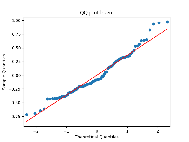
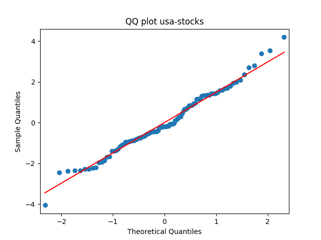
The quantile-quantile plot of earnings growth (nominal and real) versus the Gaussian distribution for Model 0:

The quantile-quantile plot of earnings growth (nominal and real) versus the Gaussian distribution for Model 1:

The quantile-quantile plot of earnings growth (nominal and real) versus the Gaussian distribution for Model 2:

The quantile-quantile plot of earnings growth (nominal and real) versus the Gaussian distribution for Model 3:

Conclusion: Unfortunately, residuals are independent identically distributed but not Gaussian, for each of the four models. Still, we need to pick one. Let us pick Model 2: Volatility is not significant, as shown by the Student test. Although it is not quite applicable, since residuals are not Gaussian! Let us write this equation after multiplication by the volatility:

See https://github.com/asarantsev/growth-spread for code and data.

Model explanation: Continuing research by Ian Anderson with updated data, 1927-2024, consider the following model for and which are spreads BAA-AAA and BAA-Long. Here, AAA and BAA are Moody’s December daily average rates, and Long is 10-year Treasury December daily average rates. In the previous post, we discussed that these are well-modeled as a vector autoregression of order 1, with mean reversion in the long run, if only we divide innovations and by annual volatility, computed by my other undergraduate student Angel Piotrowski. Then are independent identically distributed bivariate Gaussian.

As usual, this can unfortunately lead to ordinary least squares for regression fitting not applicable. Let us first divide each question by annual volatility, and add an intercept (constant) for completeness (because usually, linear regression includes an intercept). We get:

In the vector form, we can write this as

Results: Unfortunately, innovations here are further from Gaussian than in the previous post. Judging by the autocorrelation function plots for these innovations and for their absolute values: Yes, we can model as independent identically distributed. Same is shown by the L1 norms. But the quantile-quantile plots clearly say these are not Gaussian. Similarly, the Shapiro-Wilk and Jarque-Bera tests give us very low p-values.

Innovations	Skewness (Gaussian = 0)	Kurtosis (Gaussian = 0)	Shapiro-Wilk p-value	Jarque-Bera p-value	L1 norm for 5 lags ACF of original values	L1 norm for 5 lags ACF of absolute values
BAA-AAA	0.714	0.847	0.2%	0.4%	0.45	0.605
BAA-Long	0.631	0.181	1.0%	3.7%	0.554	0.487

We recall that the threshold 95% value for the L1 statistic is around 63%, based on Monte Carlo simulations.

Dependence upon volatility which corresponds to the term is positive and very significant. The Student T-test gives us For both regressions,

Removing intercepts: If we do the vector model above without , we get much improved innovation sequences. Compare L1 norm values:

Innovations	Skewness (Gaussian = 0)	Kurtosis (Gaussian = 0)	Shapiro-Wilk p-value	Jarque-Bera p-value	L1 norm for 5 lags ACF of original values	L1 norm for 5 lags ACF of absolute values
BAA-AAA	0.5	0.819	2.8%	3.4%	0.375	0.342
BAA-Long	0.204	-0.203	15.9%	65.8%	0.489	0.528

The p-values for Student T-test for BAA-AAA with factor BAA-Long is 32.3% and the other way around is 43%. In principle, we could model these two spreads as separate autoregressions of order 1, but with correlated innovations.

Conclusion: For bivariate vector autoregression of order 1 applied to BAA-AAA and BAA-Long spreads, dividing innovations by volatility makes them independent identically distributed Gaussian. After that, adding this volatility as a factor in a linear regression improves the fit as judging by significant dependence, and keeps innovations independent identically distributed, but destroys their normality.

Data description: This research is an improvement of Ian Anderson’s research. See GitHub/asarantsev repository 4rates, which contains Python code, Excel data, and all generated pictures. We take four series of USA bond rates, annual end-of-year (December, monthly average) data:

• Short: 3-6 month government yields 1927-1933, 3-month 1934-now
• Long: long-term government yields 1927-1963, 10-year 1964-now
• AAA Moody’s
• BAA Moody’s

We need to take this because this is an improvement over existing Robert Shiller’s data: Hard to find long and short-term interest rates. Also, Robert Shiller’s data is average January, and our data is December. But to model next year’s stock returns, we need the data we know by the end of this year: Thus we need December, not January.

Statistical Methodology: For each series, we fit an autoregression of order 1: We analyze innovations for Gaussian IID. Next, we divide for annual volatility available for 1928-2024, and analyze for Gaussian IID.

Analysis for Gaussian IID is performed as follows:

1. Skewness (with Gaussian = 0)
2. Kurtosis (with Gaussian = 0)
3. Shapiro-Wilk normality test
4. Jarque-Bera normality test
5. Quantile-quantile plot versus the normal distribution
6. L1 norm for autocorrelation function for original values, 5 lags
7. L1 norm for autocorrelation function for absolute values, 5 lags
8. Autocorrelation function plot for original values
9. Autocorrelation function plot for absolute values

For items 1, 2, 6, 7, we use the Monte Carlo simulations giving us 95% and 99% percentiles. This allows us to make normality tests and white noise tests.

Analysis of rates: We summarize results in the table below. The sign XXXXX shows we have independent identically distributed Gaussian innovations. If we have only one of two features: Gaussian but not independent identically distributed, or vice versa, we show it. The term Success means Independent identically distributed Gaussian.

Rate	Original innovations	Normalized innovations
BAA	Independent identically distributed	XXXXX
AAA	XXXXX	XXXXX
Long	XXXXX	XXXXX
Short	XXXXX	XXXXX

Thus we can use autoregression only for BAA rates: Here the for the Student T-test. Here are independent identically distributed but not Gaussian.

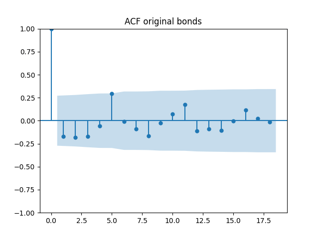
Also, we apply the vector autoregression of order 1 for the vector of all four rates. Then we apply the same analysis to each of the four series of innovations. Unfortunately but not surprising, we have complete failure for all innovations. First, we present the autocorrelation and cross-correlation function plots for these four series.

Seems like all plots correspond to white noise. But plots of absolute values of innovations show our failure. We summarize:

Rate	Original innovations	Normalized innovations
BAA	Independent identically distributed	Independent identically distributed
AAA	XXXXX	XXXXX
Long	Gaussian	XXXXX
Short	XXXXX	XXXXX

Bond spreads: Finally, we do the same analysis for spreads. There are six series of spreads.

Spread	Original innovations	Normalized innovations
BAA-AAA	Independent identically distributed	Success
AAA-Long	Independent identically distributed	Gaussian
Long-Short	Independent identically distributed	XXXXX
BAA-Long	Independent identically distributed	Success
BAA-Short	Independent identically distributed	XXXXX
AAA-Short	XXXXX	XXXXX

Let us write autoregression for BAA-AAA, AAA-Long and BAA-Long (all Student p-values are very small):

BAA-AAA: and

AAA-Long: and

BAA-Long and

Vector autoregression for two spreads BAA-AAA, BAA-Long: We write vector autoregression for bivariate series which is BAA-AAA, BAA-Long:

Overall, it seems reasonable for us to model as independent identically distributed. See below the autocorrelation and cross-correlation plots. The correlation of its two components is 89%.

Below see plots for the first series of residuals before normalization: the quantile-quantile plot versus the normal distribution; the autocorrelation function for ; the autocorrelation function for We see it is reasonable to model as independent identically distributed but not Gaussian.

Next, we normalize these residuals by dividing them by and make the three plots for We see it is reasonable to model as independent identically distributed normal.

Similar results are true for . Make the three plots for this second series of residuals.

And make the same plots after division by

Conclusion. We can model [BAA-AAA, BAA-Long] as bivariate mean-reverting vector autoregression of order 1 with bivariate Gaussian innovations. All other rates and spreads do not allow autoregression modeling with Gaussian innovations.

Of course, the spread between BAA rates and AAA rates is smaller than between BAA rates and long-term Treasury rates.

I wrote about this manuscript in a previous post. It was returned for review after two years. This is a very long time.

I updated it with new data from 2023 and 2024, corrected some misprints, and returned it to editors and reviewers for further review. I hope it gets published soon.

Luckily, this new data did not change any of my conclusions:

• This new valuation measure takes into account the difference between total returns and fundamentals growth.
• This measure works best if we take trailing averaged earnings: Innovations for the autoregressions are independent identically distributed and Gaussian.
• We picked 5 years as averaging window, but this works well also for 10 years, which corresponds to the classic Shiller cyclically adjusted price-earnings ratio (CAPE).
• The classic Shiller CAPE measure shows that the market is currently overvalued: The current ratio is much higher than the historical average or median.
• But our new valuation measure is about equal to the historical average. Thus it shows that the market is fairly valued.

I plan to write yet another manuscript to include annual volatility, see a previous post.