My Finance

Continuing research of the four bond rates, we model normalized total returns of S&P (nominal or real) as a regression upon the BAA rates at the end of last year, and the change in BAA rates throughout this year. See a GitHub repository.

Description: Let be nominal or real total returns during year Let be the annual volatility during year Let be the BAA rate at end of year

We consider two models, both for the nominal and the real versions of returns.

Model 1.

Model 2.

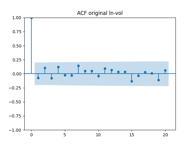
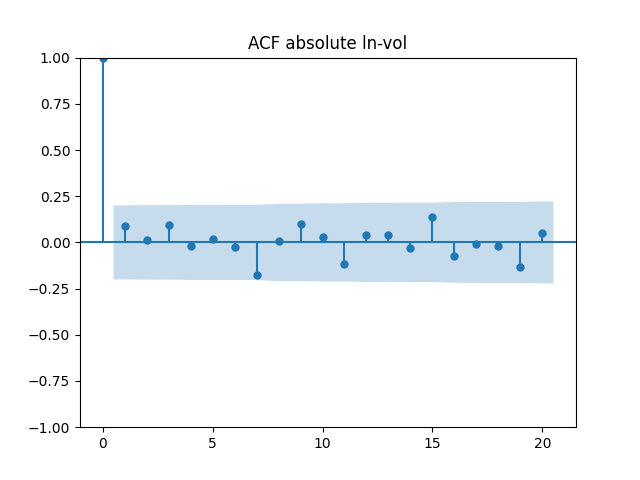
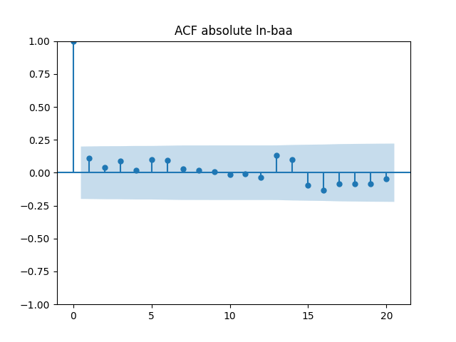
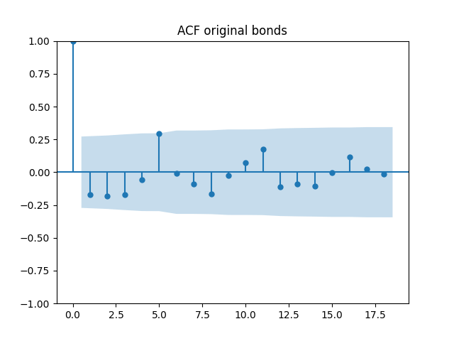
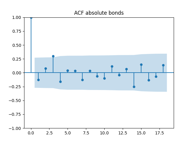
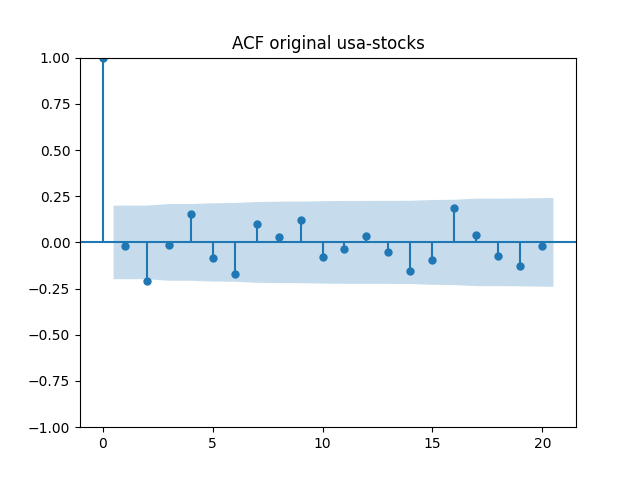
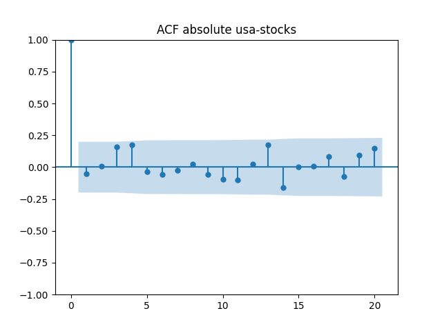
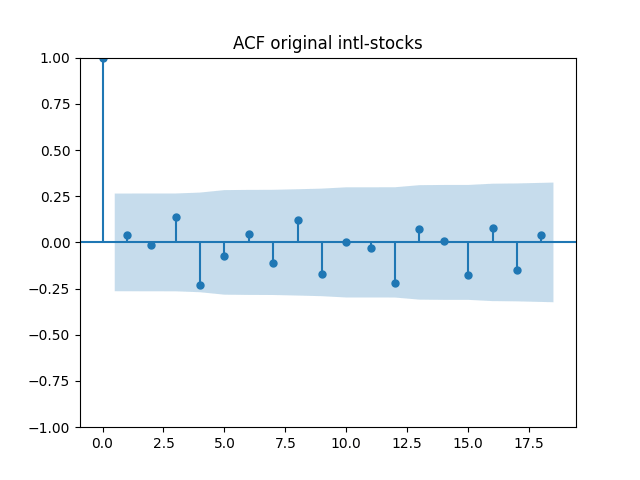
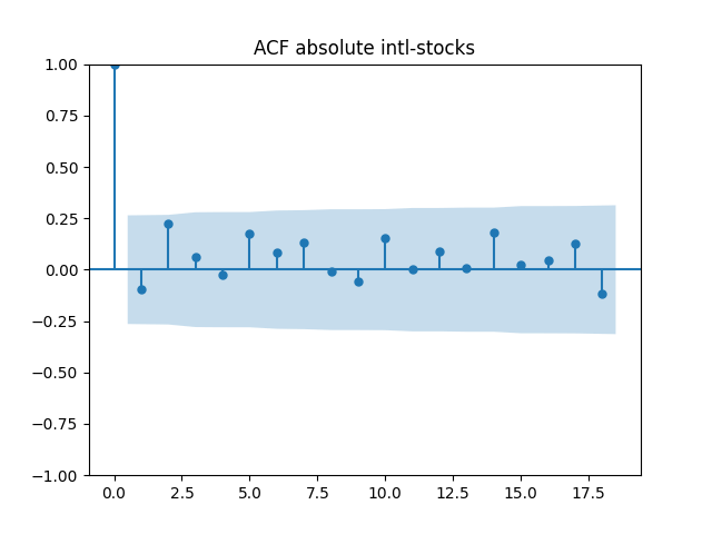
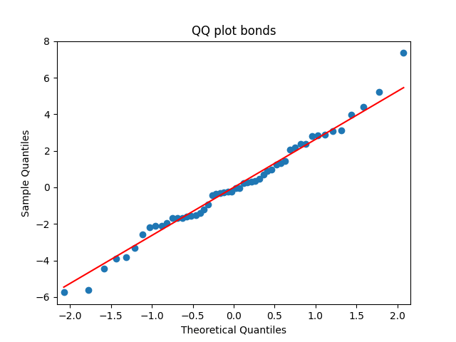
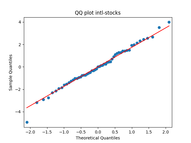
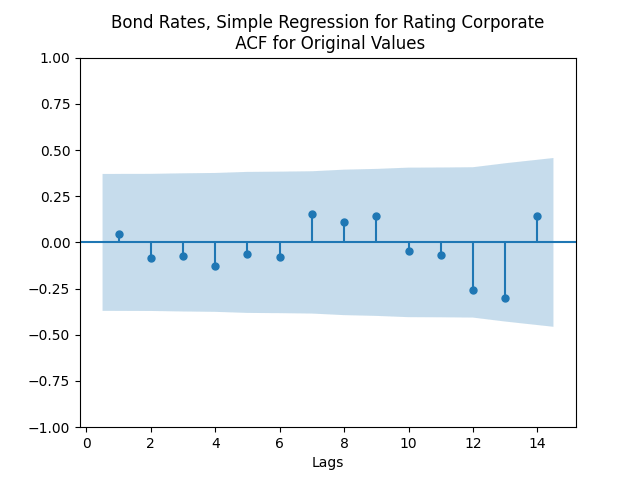
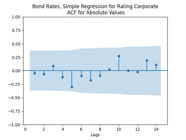
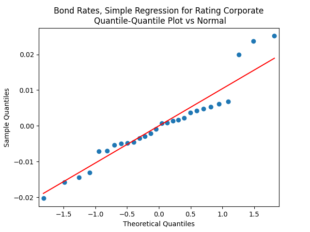
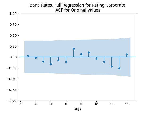
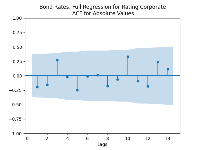
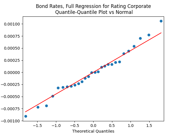
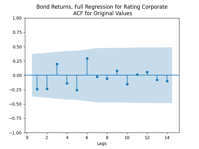
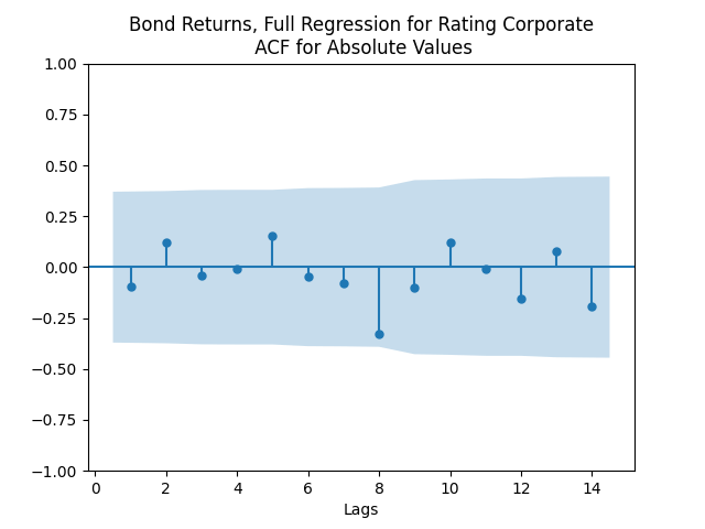
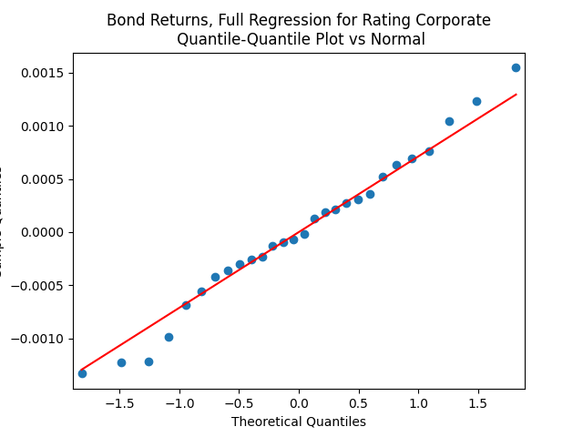
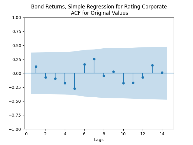
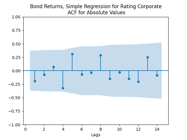
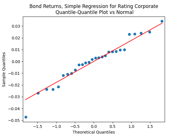
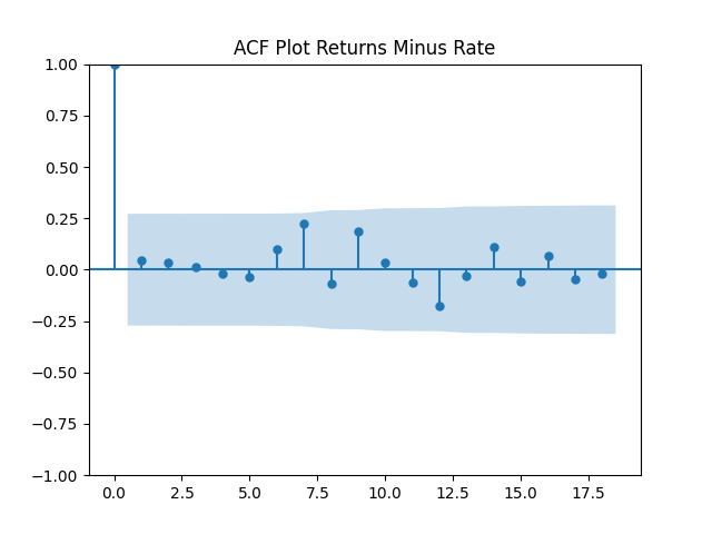
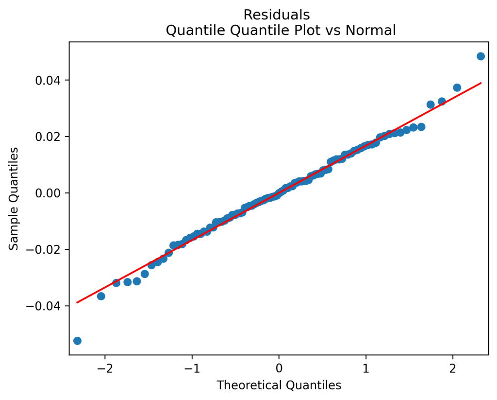
Results: In each of the four models, residuals are IID Gaussian, judging by the normality tests and the autocorrelation function plots.

But what is the goodness of fit? We get for nominal Model 1 and for real Model 1. But for nominal Model 2, and for real Model 2.

Regression results are: The coefficient is insignificant judging by the Student T-test, but is significant. In both versions of Model 2, significantly different from zero. For Model 2, actually for the nominal version and for the real version.

Conclusion: We prefer Model 2, when the is much higher.

We found a connection between Moody’s BAA bond rates and investment-grade corporate bond returns (measured by a Bank of America wealth index) Also, BAA bond rates are well modeled by a simple autoregression. This enables us to model both large stock returns and corporate bond returns. Previously, we modeled large stock returns (measured by S&P) using annual volatility and the new valuation measure. We also used bond spreads but not rates, including them in our model. Our next actions are:

• Replicate this blog with real corporate bond returns, after adjusting for inflation. We will replace (nominal) bond rates with real rates: Subtract past year’s inflation from the end of past year rate. This will be enough for an autoregression of rates. But for bond returns, we might include both nominal rate and inflation rate. Update: We failed to do this, since for the simple regression of real returns minus real rates vs duration. This is too low, and adding volatility does not improve this. See the GitHub/asarantsev repository Corporate-Bonds-Annual-Data. To be fair, residuals are IID normal for all these regressions, but this doesn’t matter.
• We need to model inflation separately, presumably as an autoregression process with volatility: If is the inflation rate in year then try or Update: We used data 1928-2024 and failed. All autocorrelation plots are unacceptable, and residuals never follow normal distribution. All normality tests fail, and the autocorrelation function L1 norm for first 5 lags are not compatible with IID assumption. See the GitHub/asarantsev repository Inflation-Modeling-1928-2024 for data and code. Strange, because we have both nominal and real returns divided by volatility modeled as IID Gaussian. So the difference between them: inflation/volatility should be IID Gaussian.
• Include these rates in the new valuation measure modeling of stock market returns. For real returns, pick real rates. for nominal returns, include nominal rates. Or maybe include both rates, real and nominal? Equivalently, include nominal rate and last year’s inflation.
• Is the distribution of residuals important? (a) simulate using kernel density estimation with Silverman’s bandwidth. Unfortunately, we cannot rely on existing functions in Python: They can only make identity covariance matrix of simulated data. (b) simulate using multivariate normal distribution with covariance matrix estimated from the data. Then compare average total returns. This will answer the second question from this post.
• Add small stocks to our research, replicating this manuscript. We can then fix capitalization ratio to the benchmark, for example 10 times smaller capitalization than S&P 500.

Then we need to update the simulator accordingly. First, we create a complete version in Python, when we can change initial values and the simulation of residuals. Second, we create a simplified version of this simulator as a web app. We will have two sliders: (a) Stocks size; (b) Bonds vs stocks.

We could make a similar slider for bond ratings, but it’s hard to quantify bond ratings similarly to stock size.

This post is continued from the previous post, which in turn continues the two posts of annual Bank of America-rated bond rates and returns. We fit the 1996-2024 data for corporate bond returns and rates.

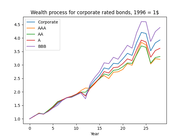
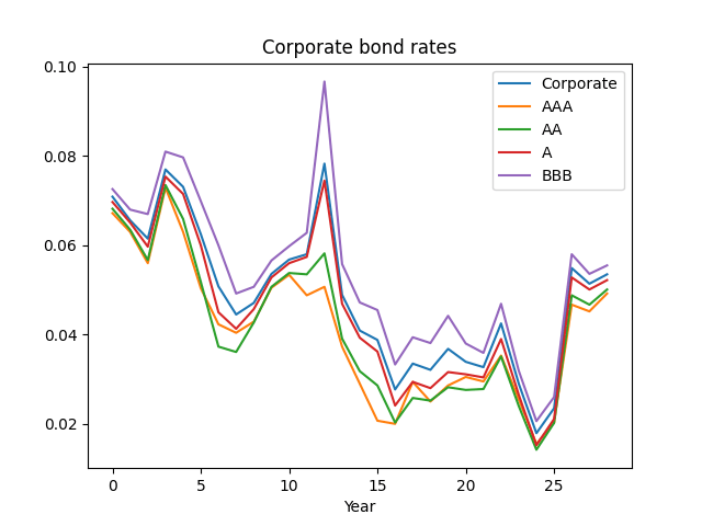
Here, we talk about investment-grade corporate bonds in general, combining all four investment-grade ratings: AAA, AA, A, BBB. Below see the graph of these corporate bond rates, together with rates of each ratings of investment-grade bonds: AAA, AA, A, BBB. We see that investment-grade rates are closer to A or BBB, rather than AAA.

Next, plot the wealth. Then we see the same pattern. We are curious why investment-grade corporate bonds behave closer to lower-rated investment ratings, rather than AAA? Maybe there are not so many AAA rated bonds.

This might be the reason why in this post AAA rates do not predict corporate bond returns very well. Remember, we have data for Bank of America bond rates only from 1996 (end of year).

We have Bank of America investment-grade corporate bond returns starting from 1972. This discrepancy gives us motivation to use end-of-year weekly data for Moody’s AAA or BAA (which corresponds to BBB in Bank of America ratings) available from 1962 to predict investment-grade corporate bond returns. This gives us motivation to replace AAA with BAA Moody’s rates.

Using the cut data from 1996, we replicated results of annual Bank of America-rated bond rates and returns. The results are the same as for AAA, AA, A, or BBB. Using annual volatility makes the two regressions have IID Gaussian residuals. All is good, except the rates are available only from 1996.

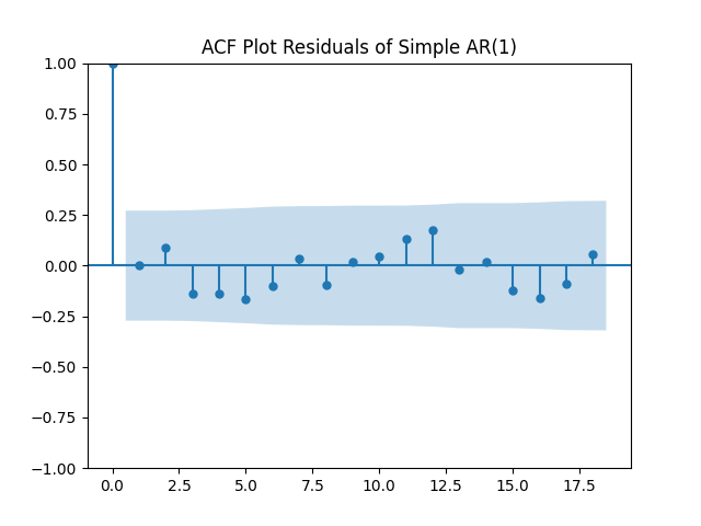
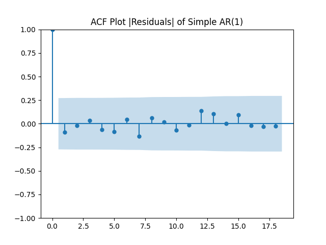
Here analysis of simple autoregression residuals for rates show they are IID but not Gaussian.

But autoregression with volatility: show these residuals are IID Gaussian. The and coefficient estimates are The Student T-test gives us for for and for The Jarque-Bera and Shapiro-Wilk The L1 values for original and absolute values of the autocorrelation function are

Model total bond returns using duration: We see residuals below.

But for the simple regression without volatility we get the following residuals:

Both regressions actually have IID Gaussian residuals, judging by Shapiro-Wilk and Jarque-Bera normality tests, and the L1 values for autocorrelation function. For the simple regression, and The value of See the Python code and Excel data (updated) at https://github.com/asarantsev/Annual-Bank-of-America-Rated-Bond-Data

Next, let us replicate results of this blog post for BAA instead of AAA rates. We uploaded updated code to GitHub/asarantsev repository Corporate-Bonds-Annual-Data. We have data from 1972.

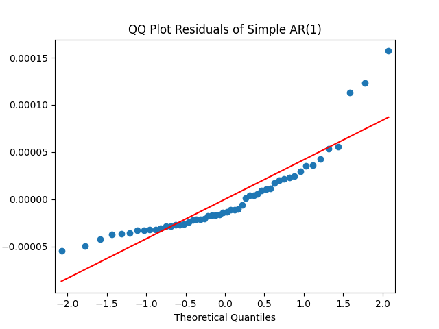
The simple autoregression for rates judging by the Shapiro-Wilk and Jarque-Bera tests, is better:

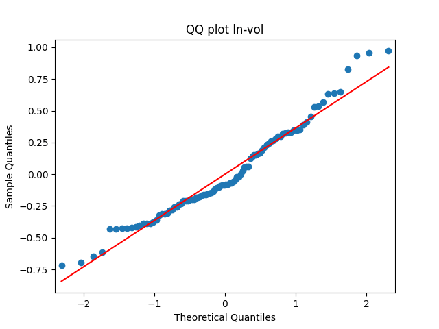
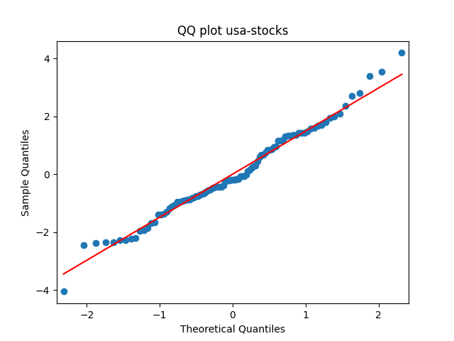
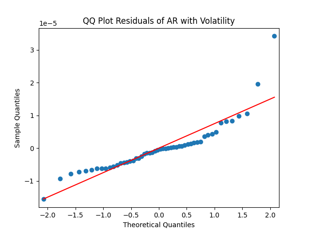
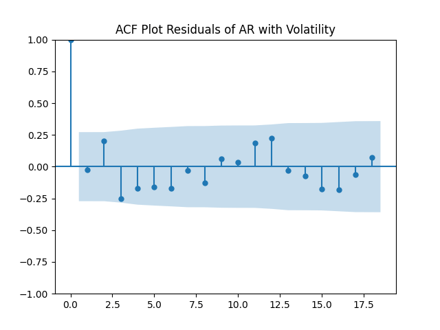
Look at residuals for autoregression for rates with volatility:

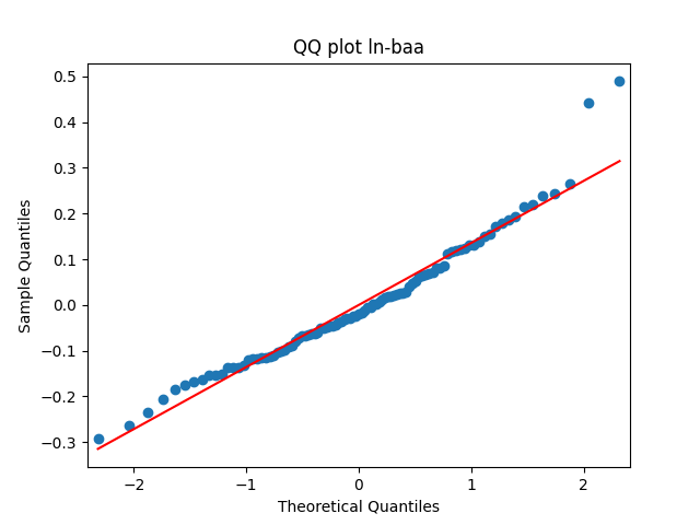
For the simple autoregression, Shapiro-Wilk and Jarque-Bera tests give us and But for the autoregression with volatility, this gives us and To be fair, from the quantile-quantile plot it is hard to tell the difference. Next, for returns minus rates if we do not regress them upon anything but simply analyze them, surprisingly, we get the IID Gaussian.

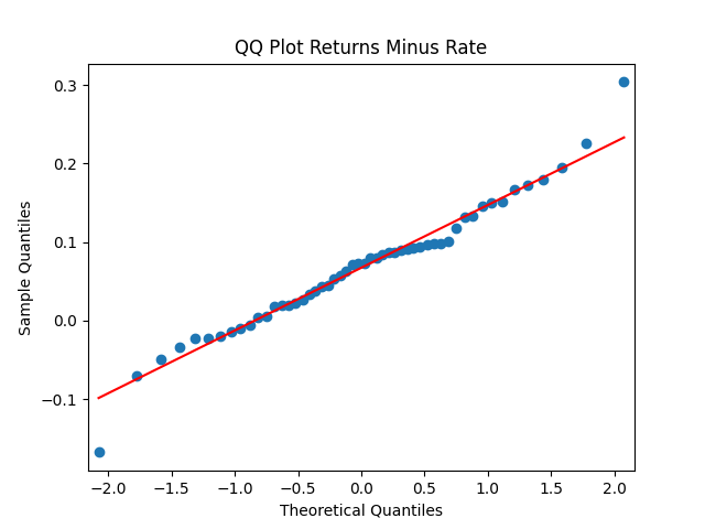
But it’s good to regress these differences upon the change in rates: We get where and And the correlation is very strong: Of course, it is statistically significant. The Shapiro-Wilk and Jarque-Bera tests give us

I updated the web site Financial Simulator and the local version on GitHub/asarantsev repository annual-simulator. I corrected the following mistakes:

• Innovations are simulated as multivariate Gaussian, since the kernel density estimator does only independent components in the multivariate case, but we do need correlated innovation series. This is very important, since independent innovations imply higher returns. The true innovations are negatively correlated. I will write more on this in the future.
• I made sure volatility from the current year not the previous year is used to model total returns. Unfortunately, I made a misprint in previous simulators. This mistake led to independent innovations instead of negatively correlated innovations.
• I removed any ability to change initial conditions, instead taking just the current conditions (volatility). I also removed any ability to change how to simulate innovations (kernel density estimation or multivariate Gaussian distribution).

Unfortunately, I made the same mistake in my other simulators.

Let me mention that I also made colored background of the plot, the legend, and the input fields. They all have different colors. Finally, I removed any references to myself and model description, because I wished to save space. I do not think usual users will be interested in this. This is only the simplest model with volatility as factor only.

TO DO LIST

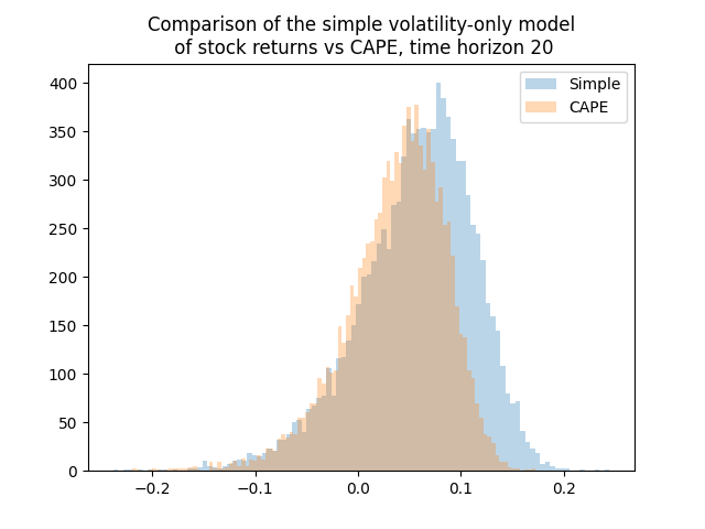
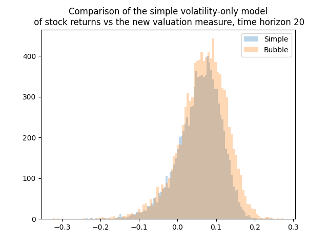
• I was thinking whether adding other factors such as the new valuation measure or bond spreads changes the distribution of average total returns or terminal wealth. Because this is the only thing we are interested in. Update: See below for comparison of the simple model, CAPE, and the new valuation measure. Yes, including earnings using CAPE or the bubble measure makes a huge difference. For current CAPE, future total returns will be lower, because CAPE is way higher than the historical average. For the new bubble (valuation) measure, the opposite is true.
• Use Gaussian vs Laplace innovations for autoregression of log volatility. Does this change the said distributions? If yes, we need to take care, and do kernel density estimation by hand. Volatility autoregression innovations are not Gaussian.
• Need to correct these misprints in the other simulators with more complicated models.

Continuing my research program, I regress S&P returns (nominal/real, price/total) upon the new valuation measure, nicknamed the bubble, and upon the three bond spreads: BAA-AAA, AAA-Long, Long-Short. We normalize this regression by volatility in the usual way. We consider averaging windows of 5 and 10 years.

Results: Each time, innovations are IID Gaussian. The ACF plots exhibit the same strange autocorrelation at lag 4. But overall, they are consistent with white noise. Each of three spreads is insignificant, judging by the Student test. But the bubble is significant for nominal (but not real!) returns, both price and total.

See the GitHub repository spreads-bubble-returns.

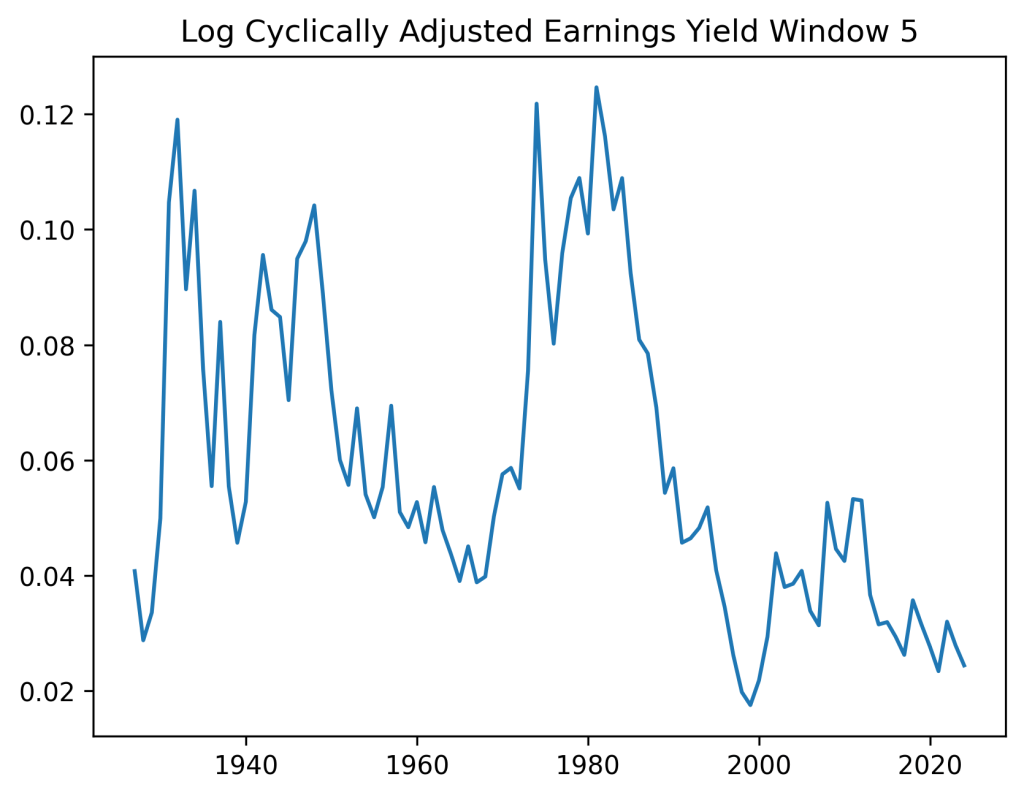
In this post, we regress annual total real returns of S&P 500 vs both new valuation measure and the cyclically adjusted price-earnings ratio (Shiller CAPE) with averaging window of 5 or 10 years. We also use, as usual, the annual volatility. Instead of this Shiller CAPE, we use its inverse, which we call simply the yield. We call the new valuation measure the bubble. We use the version of this new valuation measure at the end of that post. See GitHub/asarantsev repository https://github.com/asarantsev/New-Valuation-Measure-Replication file compare-bubble-logyield.py

The total real returns are regressed upon the bubble and the log yield end of last year. The residuals of this regression are also normalized by volatility, so we again divide the regression equation by volatility. This time, we do add an intercept, which becomes the volatility factor. Results are as follows: the autocorrelation plots of residuals and their absolute values show that these residuals are IID, see below. The quantile-quantile plot shows these are Gaussian. Same from normality tests.

The dependence of returns upon the bubble is negative (as expected) and strong, with The dependence upon the (log) yield is, surprisingly, also negative but weak, with The dependence upon volatility is negative and very strong, with The

What if we remove the yield? The new is almost unchanged, and the adjusted version is even greater after removal. This shows superiority of the bubble upon the yield as predictor.

On the other hand, removing the bubble instead of the yield reduced and the yield factor becomes a positive predictor of total returns, but statistically insignificant, with

Finally, removing both bubble and (log) yield reduced which is not much below.

The same results are for the window 5 instead of 10.

To me, it makes sense to use either yield or bubble, but not both. This applies to the model without any other factors, or with bond spreads, or something else.

I write this to combine all simulators in the same post. We consider various models for annual total returns (nominal/real) studied in previous blog posts. I carefully checked goodness-of-fit for each regression in each model, so one can trust that innovations are independent identically distributed. Unfortunately, we cannot always guarantee innovations are Gaussian. But for returns, and often for other regressions, they in fact are Gaussian. For other regressions, they are close.

In each version, we run Monte Carlo simulations 1000 times. We allow for choice of time horizon (how many years), annual withdrawals or contributions, initial wealth, and choice of innovations: multivariate Gaussian simulation (which is not exactly true, see above) or kernel density estimation. We compute the following quantities:

• Ruin probability
• Average final wealth
• The probability of the final wealth exceeding its average
• Average total returns over the paths which do not result in ruin

We also plot five paths which end in wealth ranked bottom 10%, bottom 30%, median (50% quantile), top 30%, and top 10%. This way we give a range of all plausible outcomes. I think that plotting 5% or 1% quantiles will give an unrealistic picture.

So far I have done the following versions:

• Volatility only, see this blog post and GitHub repository
• Volatility and trailing (log) earnings yield, see this GitHub repository file log-window.py
• Volatility and three spreads: BAA-AAA, AAA-Long, Long-Short, see this GitHub repository files only-rates-sim.py and only-rates.py
• Volatility, three spreads, and trailing log earnings yield, see this GitHub repository files simulator.py and 3spreads-CAPE-returns.py
• Volatility and the new valuation measure, see this GitHub repository file new-measure.py

For some but not all, I allowed initial conditions to be changed. I think it’s the best to allow index level, bond spreads, and volatility but not earnings to change. Earnings are trailing, they are a bit hard to find online, and they are updated infrequently. But the other information is updated daily.

Future work will include:

• Allowing these initial conditions (index, spreads, volatility) to be changed by the user.
• Updating all Python files so that all use the same notation and the same data file century.xlsx.
• Upload this data file to my web page.
• Test the model with this new valuation measure and the three spreads, and create a simulator for this.
• Also include both trailing earnings yield and the new valuation measure in the same regression for returns.

We need to add the following features in this simulator: Choose actions by the investor to make sure that the following events happen with given probability

• I need a given amount in a given number of years. How much do I invest now, if I contribute only at the initial time?
• I need a given amount in a given number of years. How much do I contribute per year, if I do not invest at the initial time?
• Starting from now, I need to withdraw per year during years. Here and below, we can have so we can use this money infinitely long. How much to invest now?
• In years I need to withdraw per year during years. How much to invest now, if I invest only at the initial time?
• In years I need to withdraw per year during years. How much to contribute in each of these years?
• I have now and plan to spend it for years. How much to withdraw per year?
• I have amount now and plan to contribute/withdraw per year during years. How much will I have at the end?

This is the continuation of the research in this main post and addendum post. We remove earnings yield from regression for stock index returns. The rates-only.py code is from GitHub/asarantsev repository 3spreads-CAPE-simulator

Consider annual S&P returns (price/total, nominal/real)

Standard analysis of residuals explained in this main post shows they are well modeled as independent identically distributed Gaussian. All are not significant: Student T-test has p-values greater than 5%. The most significant (having the smallest p-values) is corresponding to the BAA-AAA spread. Exceptions: for Total Nominal Returns, has The coefficient is very statistically significant with See below the graphs for simulated volatility and spreads.

We added to this GitHub repository the entire simulator for the rates-only model (with annual volatility, of course). It is done in Python file rates-only-sim.py in the same repository. See below the graph.

Below we show one simulated path of prices and wealth. This simulation is for the case of real (inflation-adjusted) version and 20-year horizon.

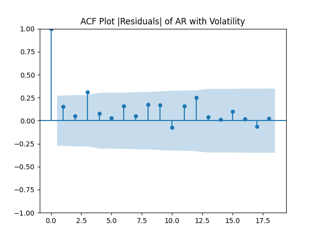
Finally, pick for the case of total nominal returns. Below we see the autocorrelation plot for , for , and the quantile-quantile plot for versus the Gaussian distribution.

As before, we have this strange value at lag 4 for autocorrelation. This presents no problem, since other values are low.

We continue part III of the blog post. There, we modeled price and total returns of S&P 500 (both nominal and real) as a linear regression with four factors: three bond spreads BAA-AAA, AAA-Long, and Long-Short; and earnings yield (last year’s earnings divided by the end-of-year index level). Look at that blog post for background and definitions.

As usual, we had regression residuals multiplied by annual volatility. Also, as usual, we added this volatility as the fifth factor. So that after dividing the regression equation by this volatility and applying ordinary least squares fit, we still have an intercept in this new regression equation.

Here, we change this classic earnings yield to its cyclically adjusted version. We allow any averaging window between 1 and 10 years.

We make another change compared to the blog post: Instead of the earnings yield as a factor in linear regression for total/price and nominal/real returns, we take the logarithm of this earnings yield. This is motivated by a remark at the end of this post.

We also add results of parts I and II in the blog post and unite them in the same Python code file. This is different from the blog post, where we split the Python code in 3 files corresponding to each part I, II, III. The code and data are on GitHub/asarantsev repository 3spreads-CAPE-simulator

Consider the linear regression

Here, are spreads: BAA-AAA, AAA-Long, Long-Short, and cyclically adjusted earnings yield (average earnings over the last few years divided by end-of-year stock index. As usual, is annual realized inflation, and are independent identically distributed. We fit this for windows of 5 and 10 years, and for which are total/price returns, real/nominal versions.

Methods: We apply standard analysis of residuals , outlined in this previous post. We also consider of this regression and compare this with cut version without any spreads. Finally, we consider the Student T-test for each coefficient.

Results: All residuals can be reasonably modeled as IID Gaussian. All coefficients in the large regression are NOT significant. The most significant (having smallest p-value) among spreads is usually BAA-AAA. Adjusted does not change much for price returns and barely for total returns.

Conclusion: This is a great model. We can use it in the simulator, which we uploaded in https://github.com/asarantsev/3spreads-CAPE-simulator

Simulation: We allowed to change the index level, three spreads, and volatility for the initial conditions. But we did not allow to change trailing annual earnings. We have an entire averaging window, we do need this, as shown in the previous research. Input of 5 or 10 annual earnings would be cumbersome for a user. However, input of current price is easy.

Also, it’s easy to look for current S&P 500 level, rates (which lead to spreads) and volatility (measured by VIX) in the market. But it’s harder to look up last few years of earnings. Anyway, these earnings change slowly and are updated rarely.

Continuing the research in the blog post and using the Python code from my GitHub repository, I made a simulator of the Standard & Poor 500 annual total returns using the new valuation measure and annual volatility with inputs: Nominal or Real, and averaging window ranging from 1 to 10 years. We can input time horizon, withdrawals/contributions, choice for innovations simulator: kernel density vs multivariate Gaussian law, and initial wealth, for the simulation. This is similar to the combined simulator for volatility and cyclically adjusted earnings yield: see this post and this post. We do not allow the user to choose initial conditions for the simulator, instead making them to be the current (as of December 2024) market conditions.

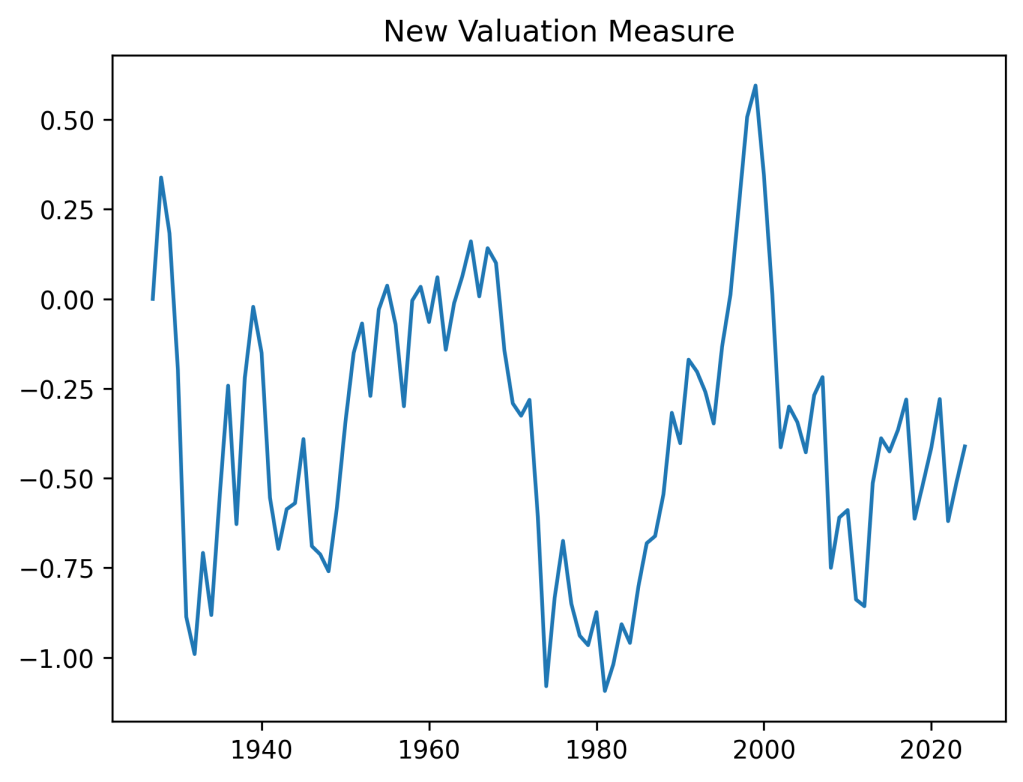
We consider the regression for where is total returns and is earnings growth terms. Let be the new valuation measure. Then we model as an autoregression of order 1: Earlier we found that it is better to model where is the annual volatility, and are independent identically distributed Gaussian with mean zero. But to use the ordinary least squares regression, we need to divide this equation by the volatility and then fit it. However, this new normalized regression does not contained the intercept

After going back to the original formulation, this intercept term would become the factor of volatility:

Comparing the two regressions, we see that can be rejected: the Student T-test gives very low p-values. This shows us that we might want to use the extended regression. But we keep the original regression with volatility but without the intercept, to make it simple. Extending it will require more research.

Below we see the results plot for this simulator. We pick 7-year averaging window and 30-year time horizon. The current measure is lower than historical average. This is the opposite of CAPE which shows that currently (as of December 2024) the S&P 500 is overvalued. We see that the variance of the terminal wealth is not very large, compared with the CAPE-volatility model with log(earnings yield) as factor instead of earnings yield in this post.

We need to do the following actions:

• Allow for a version of this simulator with 1-year earnings (no averaging) to choose the initial valuation measure and annual volatility. For 2-year and wider averaging windows we do not allow this, because picking earnings for each of 2 or more last years is too complicated for the user.
• Present a table for all averaging windows, how good is regression fit? and values for Student T-test. Are innovations Gaussian or independent identically distributed? If the regression fit is not good, according to these metrics, we can prohibit the user to apply these choices for averaging windows.
• Include the volatility in the main regression, that is, the coefficient Presumably we need to adapt the autoregression simulation for that. Also, analyze the innovations and see whether this is a good fit. If not, again prohibit the user to apply these options.

This would complete the research for earnings. But we also need the bond spread analysis. This is left for further research: To build a simulator and to include trailing averaged earnings for more than one year. But then you should not allow the user to change these earnings. Maybe it’s OK to choose volatility or bond rates (which lead to bond spreads).