1. Introduction and data description. Continue the research after updating the data for 2025. In the previous post, we discussed total returns for S&P 500 in detail. Now we discuss bond returns. We take the same data as above, and for bond wealth process , we take FRED series BAMLCC0A0CMTRIV, last trading day of year 1972-2025. We start from for the last trading day of 1972, and go on from there. This way we can compute log price returns for year
2. Relation between price returns and wealth process. We derive log price returns from this wealth process using bond math. Then we run linear regression of this log price returns versus rate change. This regression coefficient is called the duration. In continuous setting, this is defined as minus derivative of the log price with respect to the interest rate. More precisely, we use yield to maturity as this interest rate.
Wealth at end of year is and at end of year is Assuming the price of this bond at end of year is Then the coupon paid during year is The wealth at end of year is the sum of this coupon and the price at end of year Combining this, we get:
We have This gives us the formula for log price returns:
Since are observed, we can compute If we fit this model, we can rewrite
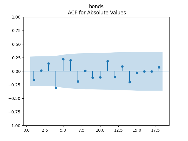
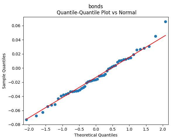
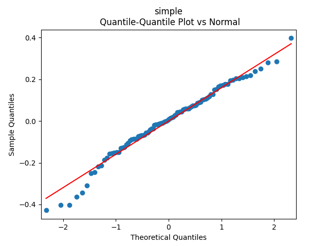
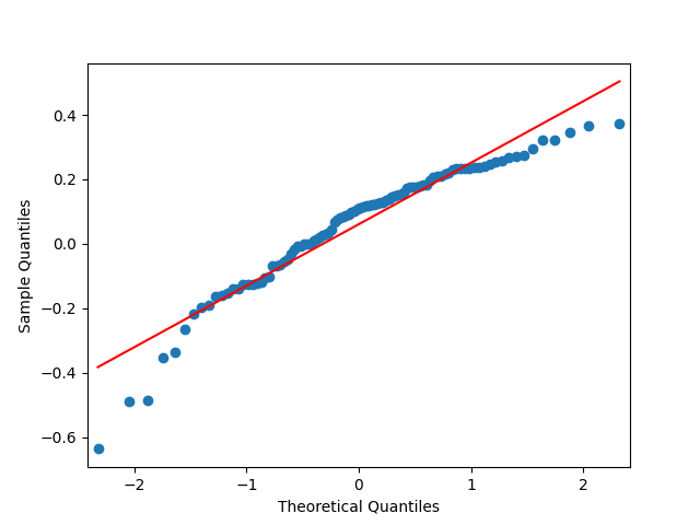
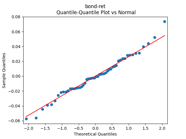
3. Fitting linear regression. As mentioned above, the log price returns can be regressed upon We do not include an intercept into this regression, since this has the meaning of a discrete approximation of a derivative. The regression coefficient is 6.1053, and the residual analysis is done by the plots below. These are Gaussian but not quite independent identically distributed. This is confirmed by the p-values of Shapiro-Wilk and Jarque-Bera normality tests: and And by the Ljung-Box test for 5 lags for original and absolute values of residuals, which give us and
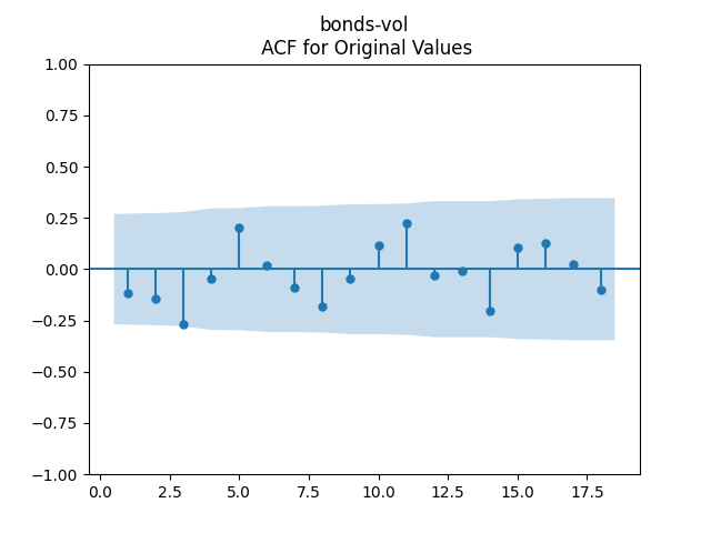
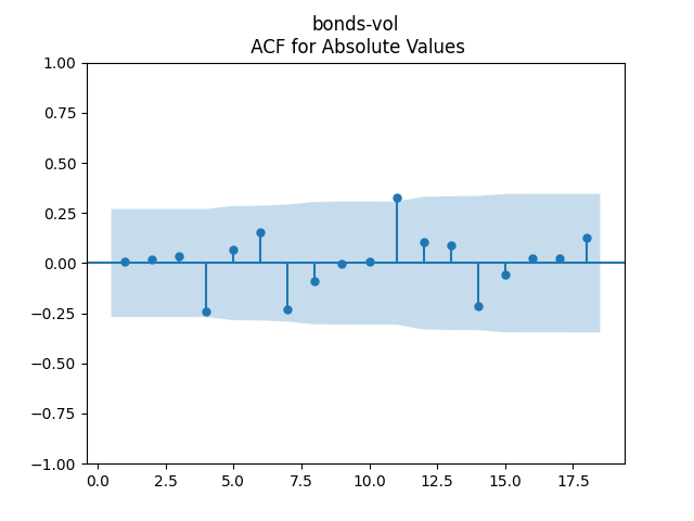
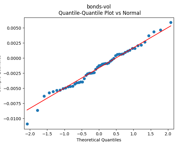
To make residuals independent identically distributed, we divide each term by annual volatility This is equivalent to assuming that the residuals are heteroscedastic: These are white noise multiplied by This gives us 5.96 regression coefficient, and for Shapiro-Wilk normality test, for Jarque-Bera normality test. Also, the Ljung-Box test for the first 5 lags of original residuals has and for absolute residuals has Finally, see the graphs for residuals below.
4. Conclusion. We have where are independent identically distributed Gaussian. We succeeded in modeling the bond market! Duration in both cases is around What is more, this is better than previous models:
We clearly explain the meaning of duration as dependence measure of the price upon yield to maturity, and not rely on approximate formulas, such as in this blog post
We used volatility in our model, but stock volatility used for bond returns is highly unusual
Residuals are independent identically distributed and Gaussian
Together with the two previous blog posts, we can now create a complete model of:
BAA rates
Dividends
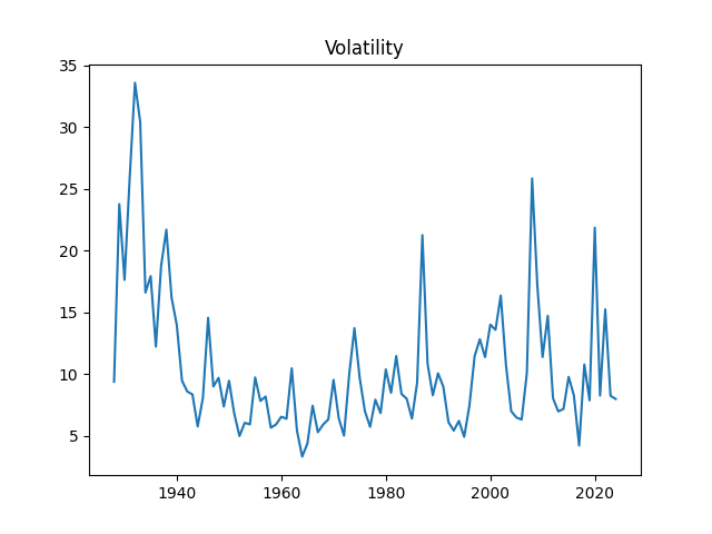
The volatility
The valuation measure
Total stock returns
Total bond returns
These are 6 time series with 5 innovation sequences. Thus we can use it to create a simpler version of the financial simulator.
1. Motivation of the new valuation measure. We continue the previous blog post. We replicate the valuation measure here. We use updated data for 2025. Previously we did this with 10-year earnings but now we wish to do this with 1-year dividends.
We prefer dividends to earnings for the following reasons:
Dividends are the actual cash paid, and they are not disputable, but earnings depend on accounting standards
Dividends are more predictable, since companies do not like to cut them, but earnings are highly volatile
Earnings of companies can be negative, and thus suffer from the aggregation bias, but dividends are nonnegative
2. Fit autoregression with linear trend as before: Take the index level at end of year and dividends paid at year Total returns and dividend growth are given by and
We model the cumulative difference as a simple autoregression of order 1 with trend: where are innovations. The valuation measure then is defined as
This can be written as We fit The autoregression becomes the random walk (there is no mean-reversion) if but this hypothesis has which is very low. Next, the trend coefficient is zero if which has
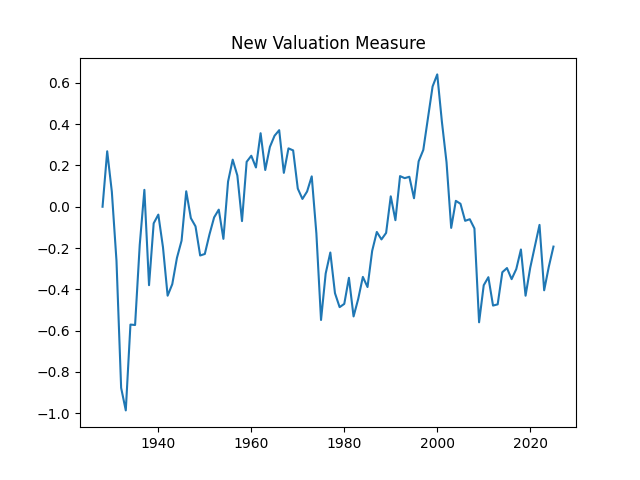
From here, we can deduce and compute the valuation measure The measure, as before, shows us that the market is not overvalued, since it is average compared to the historical standard.
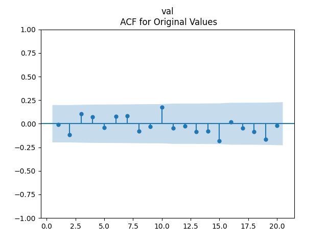
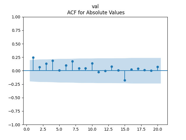
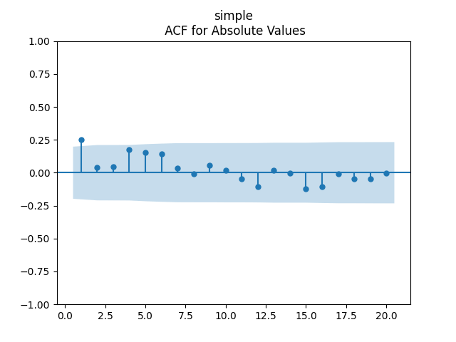
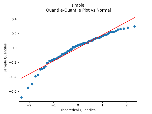
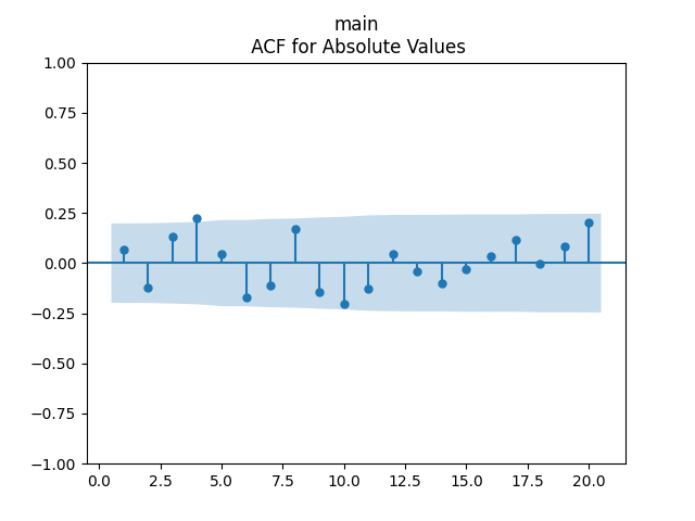
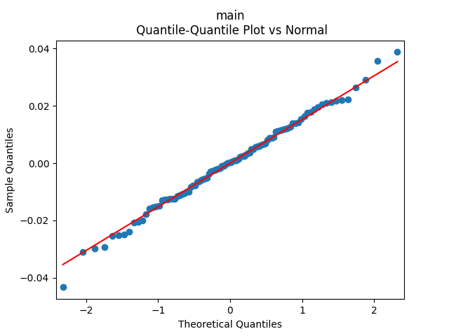
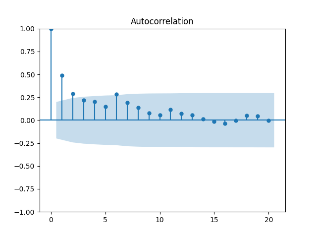
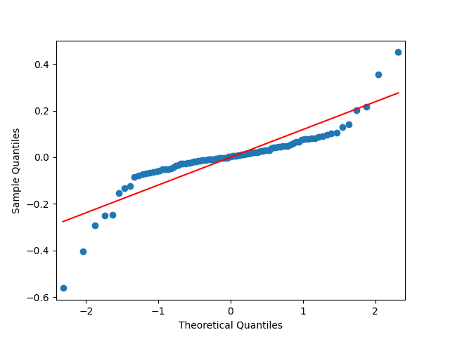
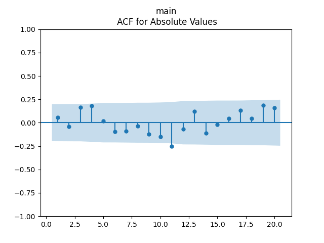
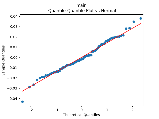
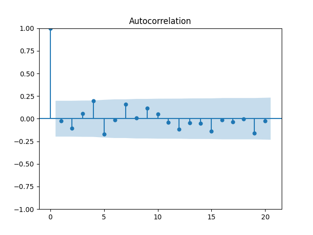
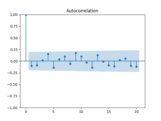
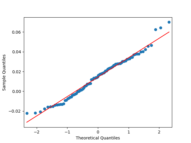
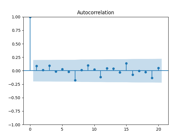
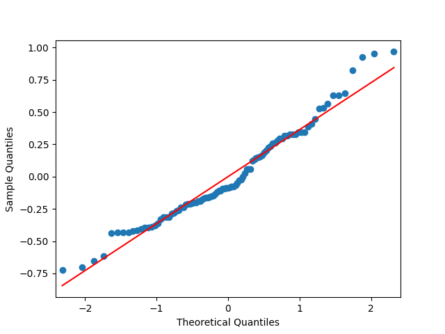
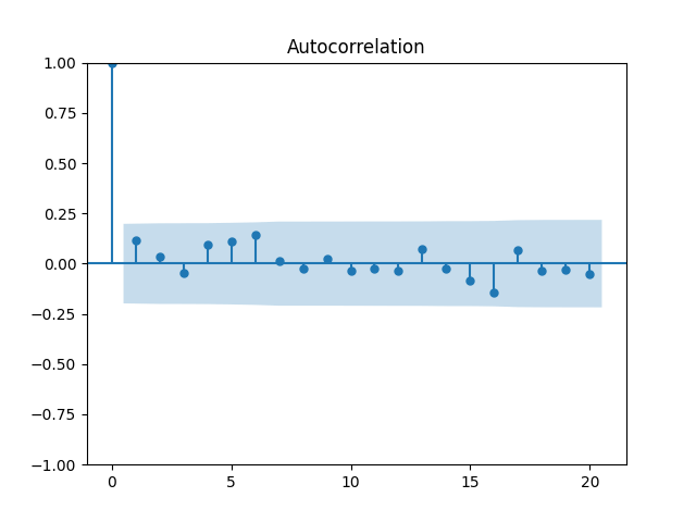
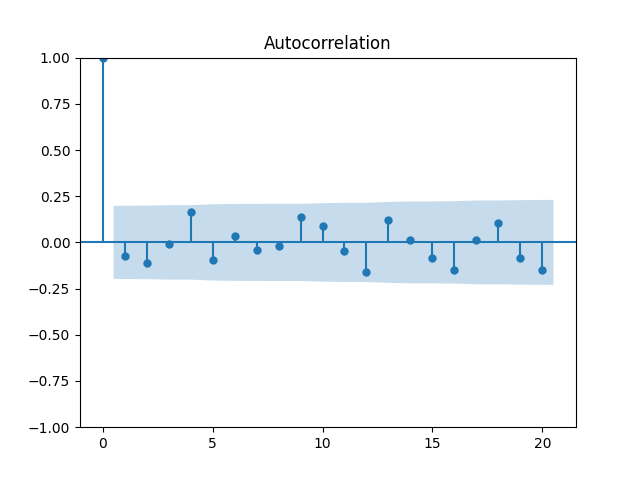
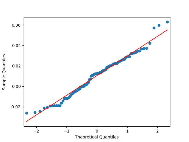
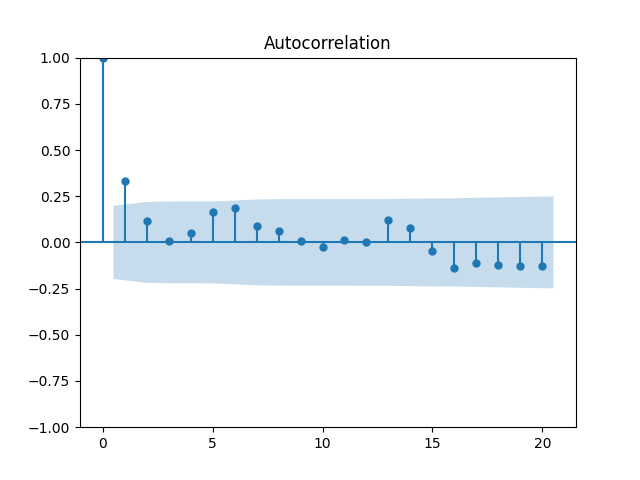
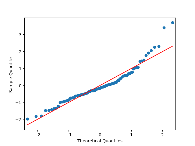
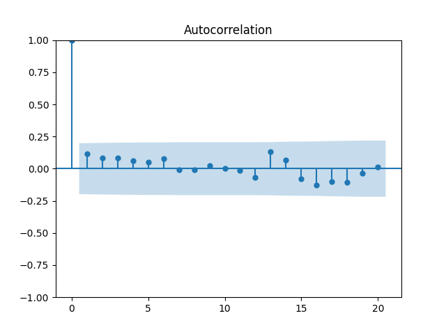
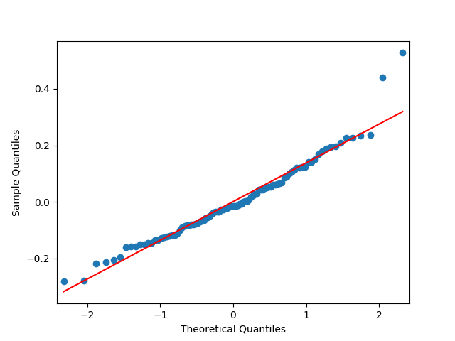
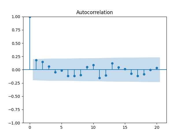
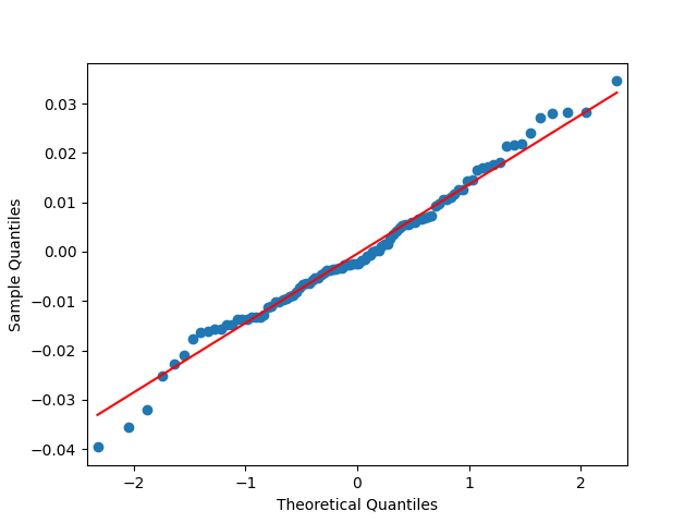
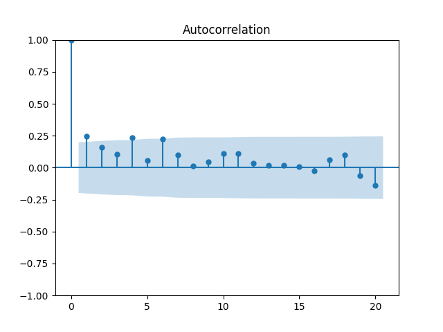
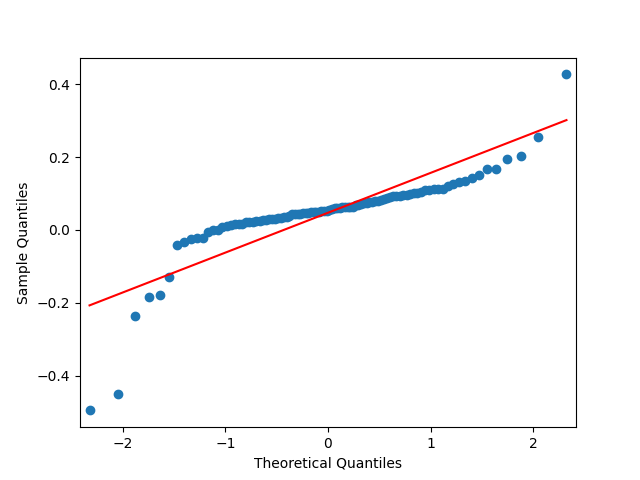
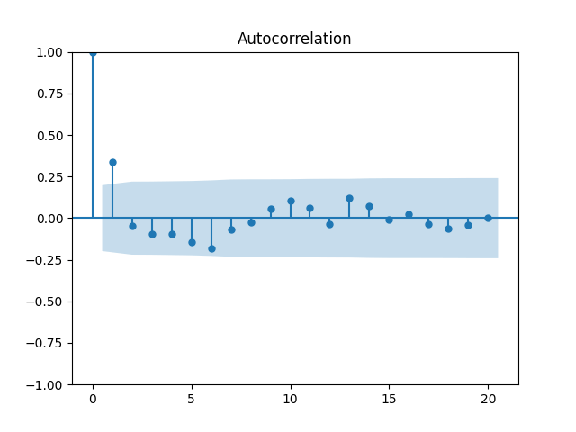
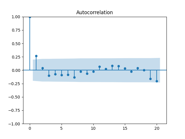
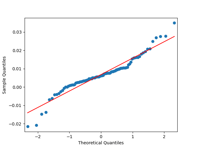
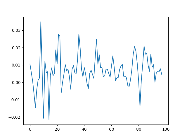
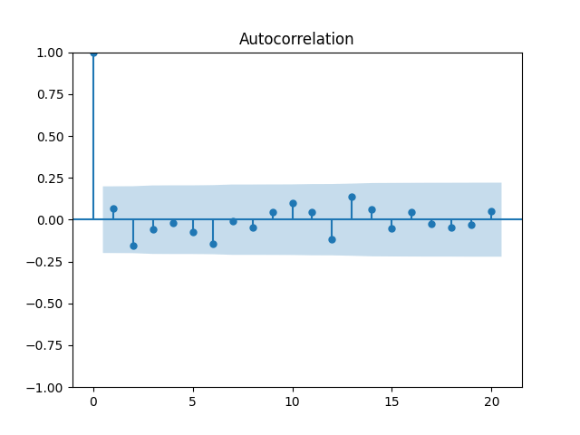
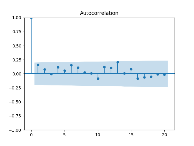
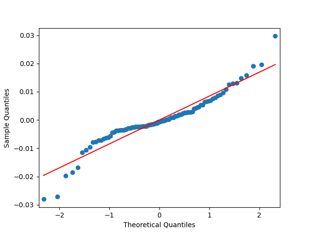
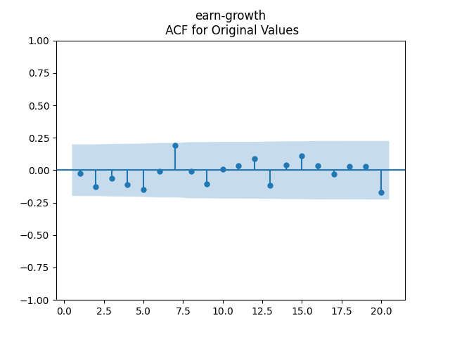
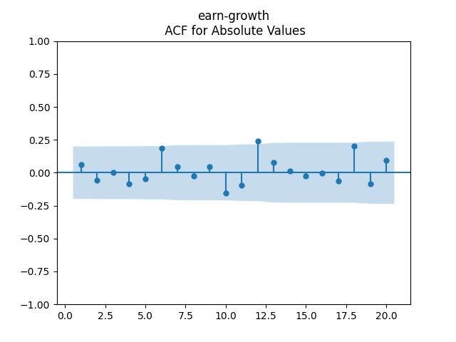
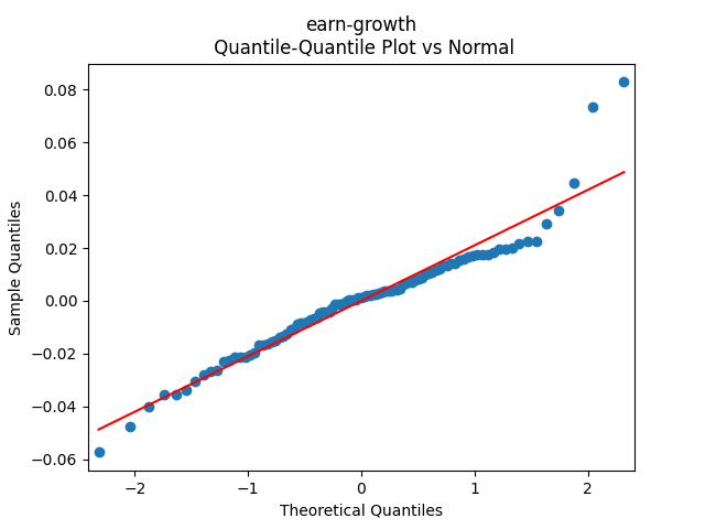
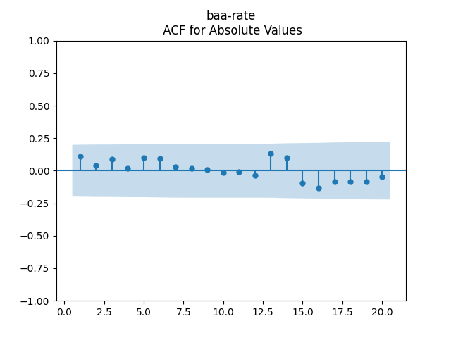
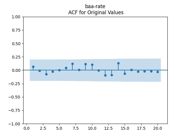
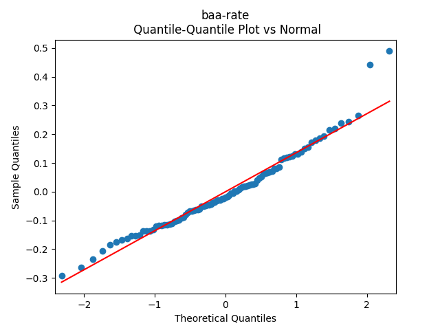
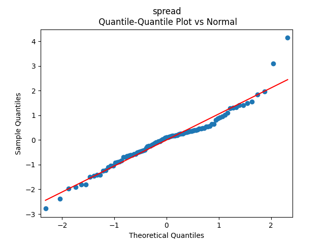
Analysis of residuals: See the autocorrelation function plots for and for as well as the quantile-quantile plot for The Shapiro-Wilk and the Jarque-Bera test give us and
We can approximately assume that residuals are independent identically distributed Gaussian, although the autocorrelation function for lag 1 for the absolute values of innovations raises questions.
3. Use this valuation measure for modeling returns. We can model total stock returns with dividends.
Model 1. Since we know how to model dividend growth from the previous blog post, together with annual volatility, we can simply model stock returns using three time series:
the new valuation measure as autoregression
volatility as another autoregression on the log scale
normalized dividend growth as yet another autoregression
Model 2. However, we can also regress upon as follows:
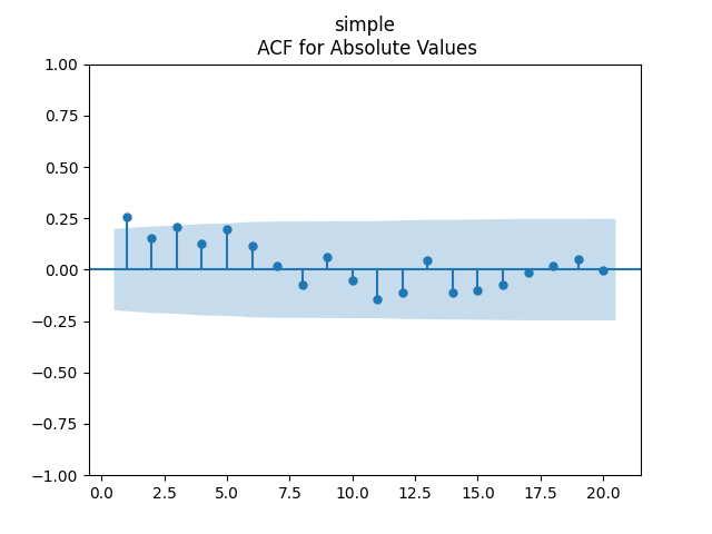
We get Also the p-value for hypothesis is The plots for residuals are below. This is independent identically distributed but not normal. Same is confirmed by the two normality tests, which give us extremely low p-values.
This model uses four time series, but with only three series of innovations:
returns regressed upon last year’s new valuation measure
the new valuation measure as the detrended difference of total returns and dividend growth
volatility as another autoregression on the log scale
normalized dividend growth as yet another autoregression
The second time series is without new innovations: Indeed, we simply write from the definition of the new valuation measure; and this does not have any new innovations. We modeled and separately.
Model 3. Let us modify Model 2 to include division by volatility: We divide by both returns and the right-hand side.
We get The p-values are all or less. The normality tests for innovations show p-values above 90% and this is confirmed by the plot below. The values of can be modeled as independent identically distributed Gaussian, therefore; see the three plots below.
This model also uses four time series but with three series of innovations, as in Model 2.
4. Include bond rates and duration. Following the previous blog post, we include rate change in our time series models. Here is the BAA rate, December daily average for year
Model 1. Try to include this rate change as a factor in dividend growth model The two other time series: the valuation measure and the volatility do not need rate change as the factor. We get:
But we run into problems: The coefficient is not significantly different from zero, with and the autocorrelation function and quantile-quantile plots for residuals shows this is not independent identically distributed and not Gaussian, see below.
Similar results are if is divided by Thus we abandon this idea of including duration (dependence upon rate change) in normalized log dividend growth.
Finally, try to include instead of This means using rate itself instead of rate change as a factor. Or normalize this rate by volatility: In each case, still we have these plots as above for regression residuals.
Conclusion: We failed to model normalized dividend growth using rate or rate change for BAA bonds.
Model 2. Include duration in the regression for total returns, together with the valuation measure:
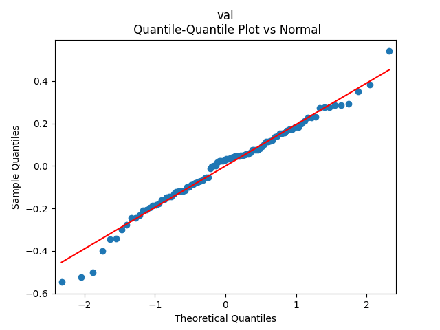
We get with p-values 8.6% for valuation coefficient zero and less than 0.1% for intercept and duration. Also, the residuals are Gaussian, with Shapiro-Wilk and Jarque-Bera normality tests giving us and But not independent identically distributed. See the three graphs below.
Conclusion: We failed to include duration in total returns modeling without normalizing by volatility.
Model 3. Include duration in the regression for total returns, together with the valuation measure:
We get a much better fit than without the duration or in Model 2: with p-values 0.4% for valuation coefficient zero and 0.1% or less for others. Also, the residuals are Gaussian, with Shapiro-Wilk and Jarque-Bera normality tests giving us and Finally, looking at autocorrelation function plots for and for we see that residuals are independent identically distributed Gaussian.
Conclusion: Here we succeeded in including the duration as a factor for regression modeling of total returns after normalizing.
5. Conclusion: We can reasonably model the new valuation measure using one-year dividends, not trailing ten- or five-year earnings, as in previous articles or blog posts. This might be better, since in previous models we used both dividends and earnings, but here we use only dividends. It is useful to include rate change as a factor in a regression for total returns, but only after normalizing, and not for normalized dividend growth. This updates our blog post. In the next post, we consider total corporate bond returns modeling using bond rates.
Dear readers, after a long break, I am back. I updated the annual volatility and other data for S&P 500 for the year 2025. The data are available here.
Data Updates
New Graphs
Total Returns
Volatility Autoregression
Price Returns
BAA Bond Rates
Dividend Growth
Conclusion
1. Data Updates. Annual volatility is computed as the empirical standard deviation of daily log changes multiplied by 1000 (for normalizing). The end-of-year price for S&P 500 in 2025 is also updated. We also add S&P 500 dividends for 2025. Now we have data on volatility for 1928-2025, on dividends for 1927-2025, and end-of-year level of S&P 500 for 1927-2025 too.
We added the dividend data for 1927 as well, to increase the number of data points. This is fine, since S&P 90 (a predecessor for S&P 500) was created in 1926, and the data is taken from Robert Shiller’s data library.
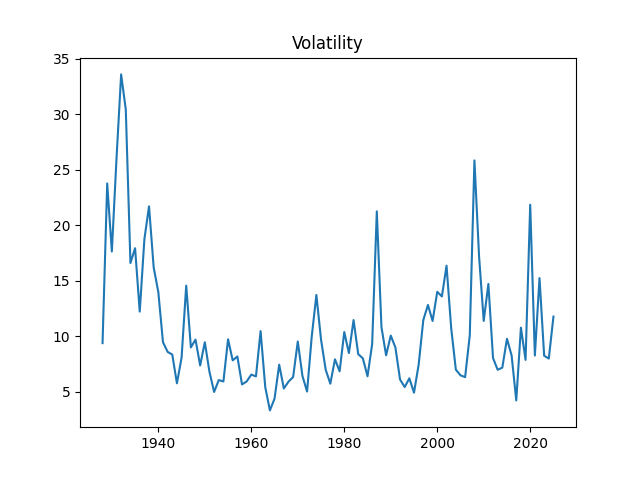
The volatility for 2025 is 11.77. This is higher than the long-term average 10.51, or the 2024 volatility, which is 7.98. See the original post with computations of Angel Piotrowski for 1928-2023 and its previous update for 2024.
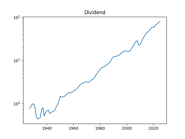
Dividends for 2025 are 78.92, which is significantly higher than dividends for 2024, which are 74.83.
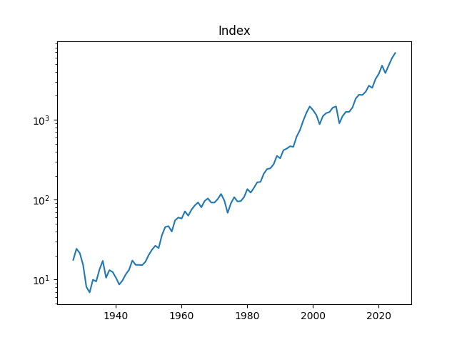
The S&P 500 increased a lot in 2025: End-of-year 2024 level is 5881.63, but end-of-year 2025 level is 6845.5.
We could not yet provide earnings for 2025, since we have earnings for 2025 Quarter 4 reported only on 2026 Quarter 1, which is still ongoing. We will provide them as soon as we can.
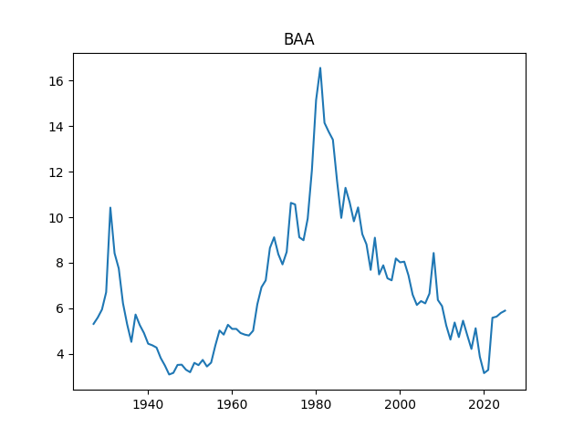
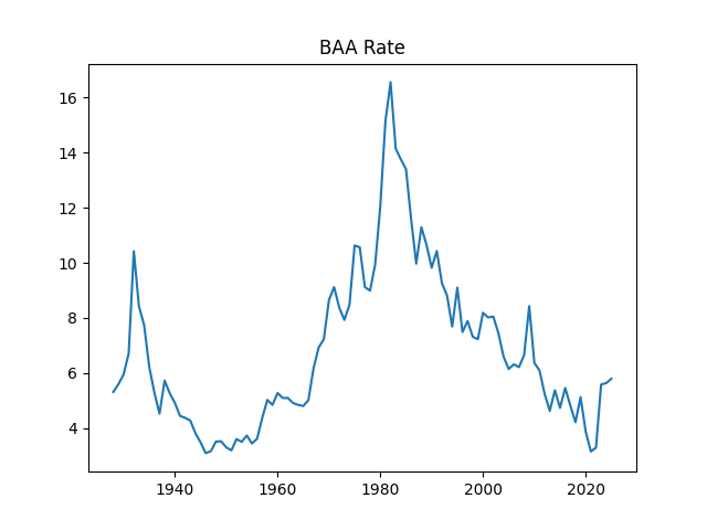
Finally, we added the BAA rate: December 2025 daily average. The BAA are lowest-rated investment-grade corporate bonds. The rate in December 2025 is 5.9, slightly higher than 5.8 for December 2024.
2. New Graphs. We graph the index, dividend, rates, and volatility.
Above, logarithmic plots of index levels and dividends for 1927-2025. Below, the annual volatility and December BAA rate.
The data are published on my web page: We created a new tab named Financial Data Library on my web page. Let us now apply
Let us replicate this post: Make stock returns IID Gaussian.
We have the following notation:
the S&P level at end-of-year
the dividend of S&P in year
December daily average BAA rate during year
annual realized volatility for the S&P for year
3. Total Returns. We continue this blog post. Compute total nominal geometric returns for the S&P 500: for year Below is the graph of returns 1928-2025.
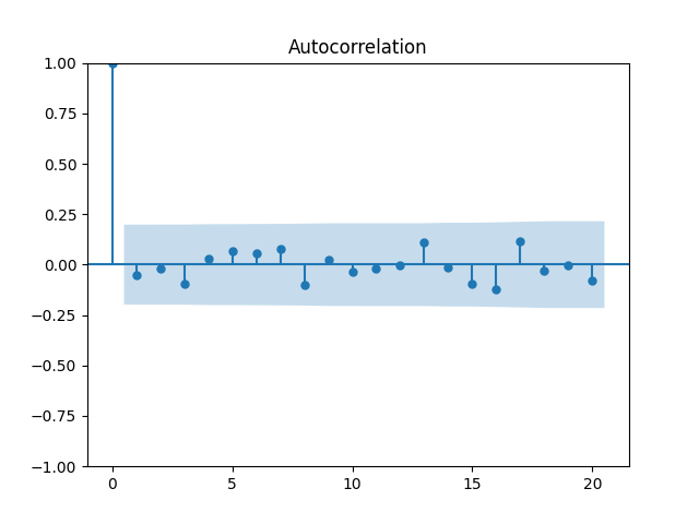
Now plot the autocorrelation function for these total returns And another autocorrelation function for their absolute values Both plots are below, and both are consistent with the white noise hypothesis. It is surprising that we, in fact, do not have to divide total returns by annual volatility to make it white noise.
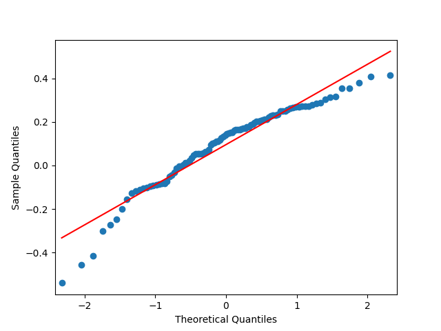
The quantile-quantile plot of these returns is shown as well. We see that the returns are not Gaussian. This is consistent with the normality testing. Shapiro-Wilk and Jarque-Bera tests give us and
What if we do divide these total returns by annual volatility? We get Let us plot the autocorrelation function for and the autocorrelation function for
These are still consistent with white noise, although, in my view, the autocorrelation function values are greater. But the quantile-quantile plot versus the normal distribution is below. We get and for Shapiro-Wilk and Jarque-Bera normality tests.
4. Volatility Autoregression. We continue this blog post. Let us now fit the auto-regression model for logarithm of volatility:
We fit and Also, plotting the autocorrelation function of and of we see:
This is consistent with the assumption that are independent identically distributed. But it is more ambiguous to assume they are Gaussian, see the quantile-quantile plot below. The Shapiro-Wilk and Jarque-Bera tests give us and respectively.
5. Price Returns. These are computed as We continue this blog post. These contain only price changes, not dividends. The autocorrelation function for these values and their absolute values is plotted below.
Quite close to independent identically distributed! Next, the quantile-quantile plot versus the Gaussian distribution: This shows price returns are not Gaussian, similarly to total returns. This is confirmed by familiar Shapiro-Wilk and Jarque-Bera tests and
Let us divide price returns by volatility. Below we plot the autocorrelation function of and of and see that this is still consistent with being independent identically distributed. Only these values are slightly higher.
The Shapiro-Wilk and Jarque-Bera tests give us and respectively. See also the quantile-quantile plot. This is much closer to normal distribution.
Finally, let us plot price and total returns together. We see that, of course, total returns are greater than price returns.
6. BAA Bond Rates. Continue this blog. We also fit a simple autoregression:
We get: and But the p-value for the null hypothesis when we have a random walk is so we fail to reject the random walk hypothesis. This is not acceptable from the financial point of view, since the random walk implies will go negative eventually. Also, consider the graphs of autocorrelation function for and for These are not independent identically distributed.
Both p-values for normality tests of innovations are less than 0.01%. The quantile-quantile plot is shown below for It is clear these are not Gaussian.
Instead, like for the volatility, let us take the logarithm:
We get and with for the null hypothesis of random walk, which corresponds to Plot the autocorrelation function for and for below:
Let us modify this to try a random walk model: are they really independent identically distributed Gaussian? Below are the autocorrelation function plots for and for which show that these are independent identically distributed.
Next, the quantile-quantile plot versus the normal distribution is much closer to the straight line than before for other models of the BAA rate. This is confirmed that the Shapiro-Wilk and Jarque-Bera tests give us and which rejects the null hypothesis but are not as small as the previous ones.
Next, try to make these independent identically distributed but non-Gaussian terms Gaussian. We do the same as in sections 1 and 3: Divide the log rate change by volatility. We get Below are autocorrelation function plots for and for
The quantile-quantile plot below shows these are Gaussian terms, and the same is shown by the Shapiro-Wilk and Jarque-Bera tests with and This was done in the spirit of this blog post.
7. Dividend Growth is computed as We continue this blog post. See below the autocorrelation function plots for and for which show lag 1, also the quantile-quantile plot.
Define and analyze it as well. The data are closer to the Gaussian distribution, with and
See the plot of the dividend growth below. It is quite volatile but not as much as the stock returns. But we clearly see the persistence: It makes sense to model dividend growth or its normalized version as the simple autoregression. This is different from annual earnings growth, where dividing by volatility makes it independent identically distributed, see this blog post.
Let us try the simple autoregression for normalized annual dividend growth
We have and with Shapiro-Wilk and Jarque-Bera normality tests give us and See the graphs below, autocorrelation for autocorrelation for and the quantile-quantile plot for
Here we have independent identically distributed but not Gaussian residuals
8. Conclusion. Here, we found all time series Markov models for dividends, price and total returns, volatility, and the BAA rates. In the next post, we will discuss updates for the valuation measure based on one-year dividends instead of trailing 10-year earnings, and regression modeling using rate change and duration, continuing this post and this post.
In the repository https://github.com/asarantsev/advanced we added another page with advanced version of the simulator, where we can pick initial conditions for model factors:
S&P 500 Annual Volatility (VIX)
S&P 500 Bubble Valuation Measure
Moody’s BAA Bond Rate
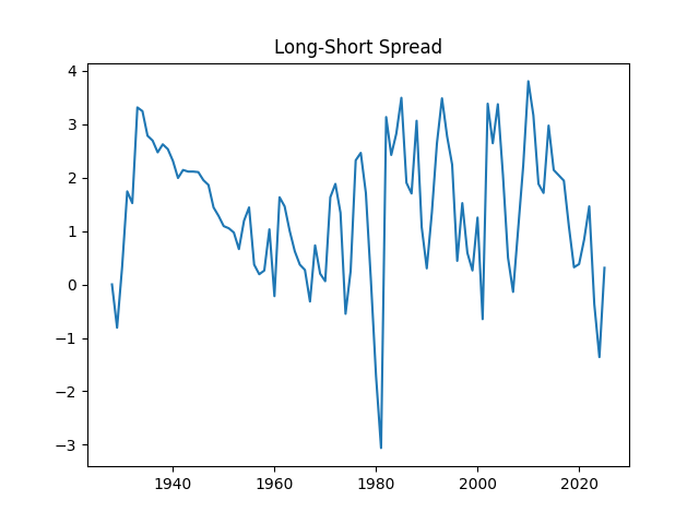
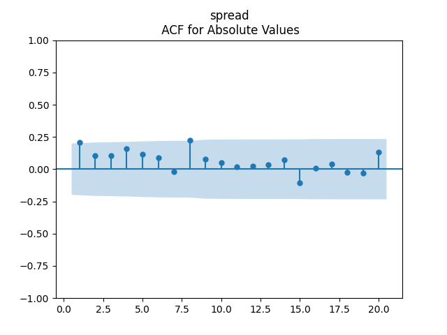
Treasury 10Y – 3M Long-Short Bond Spread
We repainted the button Compute in orange. For the advanced option, we made the legend font and the web page font smaller. And we updated the default initial conditions for the main version of the simulator to make it for June 2025.
See the historical graphs of these four measures below. We can see their historical range. We included them in the HTML page for the advanced version of the simulator.
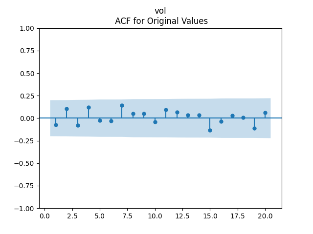
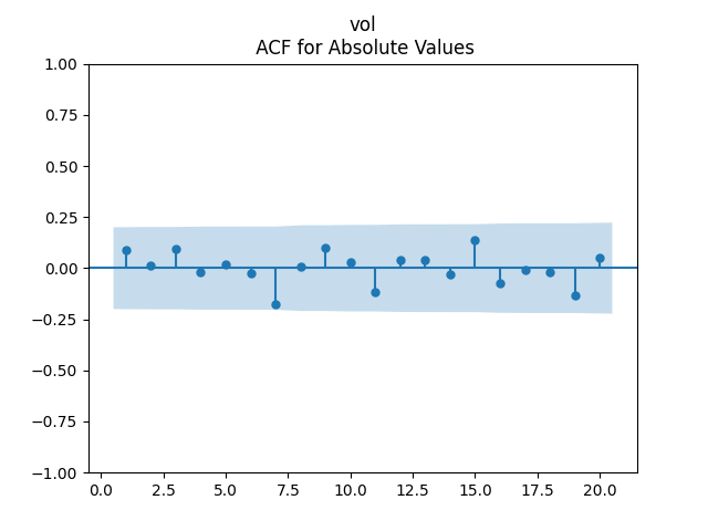
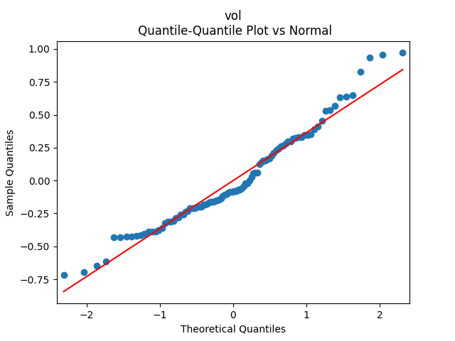
Below we see the autocorrelation function plots for original and absolute values, and the quantile-quantile plot versus the normal distribution, of residuals for each of the seven regressions. First, let us consider four factors: volatility, BAA rate, and spread (autoregressions for logarithms) and earnings growth divided by volatility (needed to compute the evolution of the bubble measure; here no regression).
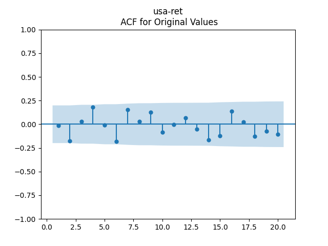
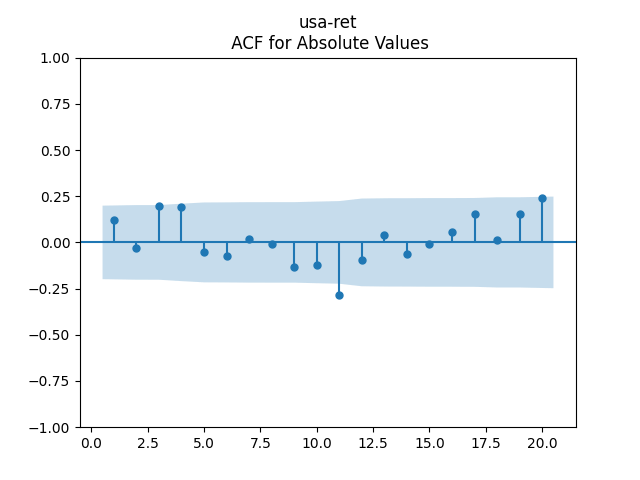
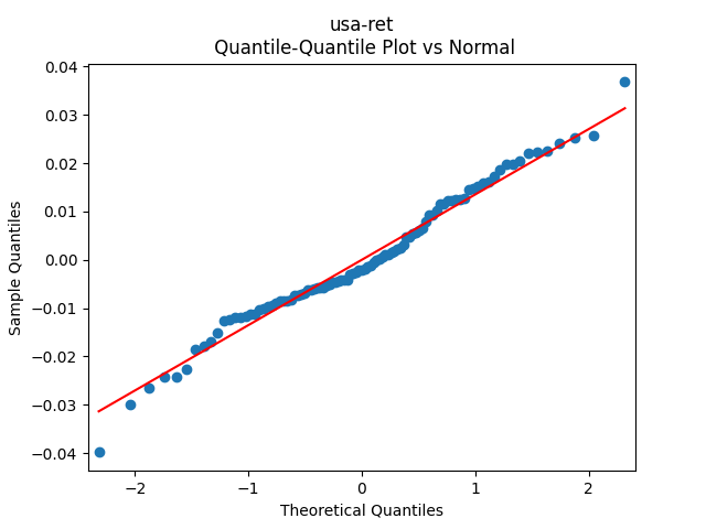
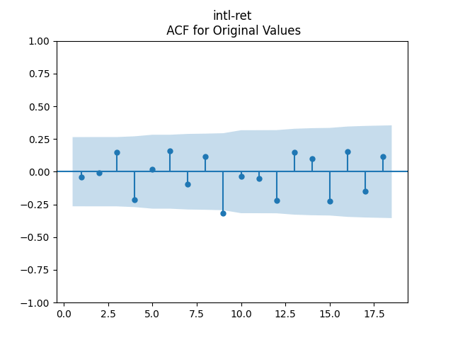
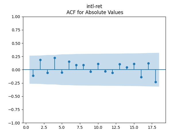
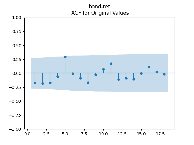
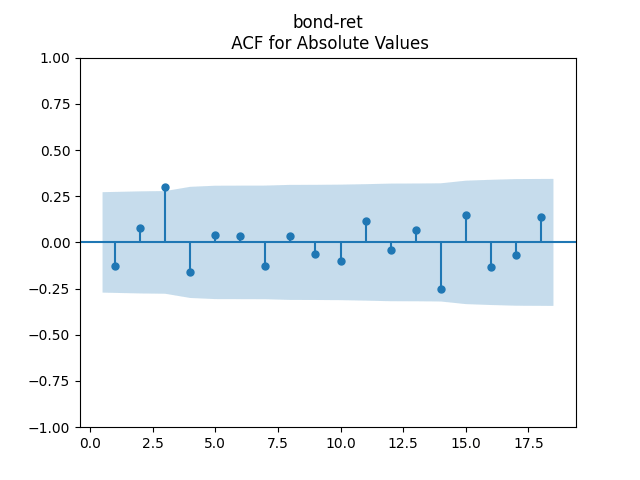
Then consider regression residuals for total returns of three asset classes: S&P 500, International Stocks, USA Corporate Bonds.
I am back! Now let me reduce the complexity of this model to model factors: log volatility, log BAA rate, and long-short Treasury spread, only using one-dimensional simple autoregressions, possibly with non-Gaussian independent identically distributed innovations. Different series of innovations might correlate.
Analysis of residuals for these is given below. You can see that residuals (innovations) are IID and close to normal.
We shall not present here all residuals analysis, instead referring the reader to the new GitHub repository, but results are almost the same as before. If I have time, I will write a detailed description of analysis of residuals. Next, we need to move to an advanced version of the simulator, which allows you to choose factor values.
I use a mix of developed and emerging markets in the portfolio of international stocks, in proportion 60/40, as in the previous version of the simulator. I use only total (not price) returns, and nominal (not real) returns. There are three asset classes: S&P 500; International stocks: 60% of MSCI EAFE (Europe-Australasia-Far East) and 40% of MSCI EM (emerging markets); and USA corporate bonds.
I modeled innovations using kernel density estimation. There are 8 regressions, but one of them (the bubble measure) is used to create said measure, not model the actual returns, so we use 7 series of residuals. I use the same algorithm discussed there to impute missing data.
For current market conditions, we use May 2025. I could write the API to take these from Yahoo Finance but I just manually put them. They need to be updated from time to time.
I put the backend Python simulation code, the original Excel file for financial data, the Python code for filling innovations series, the Excel file for innovations before and after imputation, and the HTML frontend files, to a separate GitHub repository.
This is my 50th post. And so far, the main work on this simulator has been finished, or so I hope. Now I would like to tell this as many people as possible. I am taking some break from this coding and web development. Enjoy the summer!
From the same web site Novel Investor, we included total nominal annual returns of emerging markets stocks (MSCI EM index). They are available only from 1988, as opposed to developed markets from 1970. So I added emerging markets to the portfolio in the following way: Starting from 1988, we have 60% Developed and 40% Emerging portfolio of international stocks. I fitted the econometrics model using the new data, and rewrote the simulator.
The model fits well, judging by the innovations for the regression for international stock returns. However, simulator runs show that returns have considerably increased. This is due to historical data: Returns of emerging markets were much higher than of developed markets during 1988-2024, although some years were an exception.
Regression coefficients in the model for international stock returns have changed:
Contents: Problems; Kernel Density Estimation; Missing Data
Problems. We have non-normality of innovations. Even when they are independent identically distributed, we cannot guarantee their normality. What is more, different series of innovations have different lengths. For example, in our current version of the simulator, we have five series of innovations. They are available in the Excel file innovations.xlsx in GitHub repository asarantsev/simulator-current
Autoregression for log volatility: 96 data points
S&P stock returns: 97 data points
International stock returns: 55 data points
Autoregression for log rate: 97 data points
Corporate bond returns: 52 data points
In the previous version of the simulator, I simply used the multivariate normal distribution. We can compute the empirical covariance matrix by ignoring the missing data. And the means are, of course, zero. But, as mentioned above, the distribution is not normal in fact. To be more precise, the first and fourth components are not normal. In particular, their kurtosis is greater than that of the normal distribution, and the skewness is nonzero.
I tried to apply other distributions to fit each of these two components: skew-normal and variance-gamma. But I failed to fit them well. What is more, fitting univariate distribution is not enough. I need to combine them with normal marginals for the other three components. I did not find relevant exact literature. This would require developing entire new theory of multivariate distributions.
Kernel Density Estimation. This is a universal nonparametric method: (KDE). We apply Gaussian kernel: For we have the density
where is the probability density function on for which is the dimensional Gaussian distribution with mean vector and covariance matrix In other words, to simulate a random variable with such density, we pick at random (uniformly) from and simulate the additional noise independent of Thus
For we apply Silverman’s rule of thumb: This is a diagonal matrix with
Here, are statistics of the th component of the data Namely, is the empirical standard deviation, and is the empirical inter quartile range: 75% quantile minus 25% quantile. This is realized in the file simKDE.py from our main repository. We stress that this code simulates innovations, not computes the joint density function.
Missing Data: The other problem mentioned above is lack of data for some series of innovations. We considered many imputation methods, for example iterative imputer using Principal Component Analysis or k-nearest neighbor method. They are implemented in Python package sklearn. But such methods reduce variance, because imputed data reverts to the mean. I chose a custom designed approach. It comes in iterated steps. We describe one step below.
Step. Assume we have series of independent identically distributed data points. Out of these, have full values, and the last one has missing values. We then regress this last series (of course, only existing values) versus the full series (of course, only the matching data points). We use ordinary least squares linear regression. Then we take residuals of this regression. We randomly choose with replacement of these residuals. And for each of missing points, we pick the predicted value by this regression using the first data series, and add this randomly chosen residuals. This is the way to fill the missing data. This completes the description of this step.
We first apply this step to one missing data point for series 1 (using series 2 and 4 as the backbone), then to missing data points for series 3 (using series 1, 2, 4 as the backbone), and then to missing data points for series 5. We write this new data frame into a separate Excel file called filled.xlsx. It is available in the same GitHub repository. The Python code is given in innovations.py in the same repository.
Introduction. Here I talk about improvement of my financial simulator. So far, I have the following factors:
BAA corporate bond rate, average December
Annual volatility, S&P 500
I decided to include two more important factors:
A bubble measure, which is an improvement over Robert Shiller’s cyclically adjusted price-earnings ratio (CAPE), for which he got a Nobel Prize in Economics. We discussed it here and here and here.
The long-short spread between 10-year and 3-month (average December) Treasury rates, which is often quoted as an important indicator. For example, if it is negative (inverted yield curve), then a recession is looming. We discussed it here and here and here.
We will now use annual earnings of S&P for our research. This is important, since it connects stock returns with fundamentals. This is similar to computing bond returns using bond rates. Robert Shiller used this comparison for his work. And we use this comparison to make our valuation measure. But, of course, stocks are much more volatile than bonds. So it’s harder to model.
Since we covered so much in previous posts, here we will be brief. For the person who wants to know details, we refer to GitHub repository.
Results. 1. First, recall the autoregression of order 1 for annual volatility:
Recall that
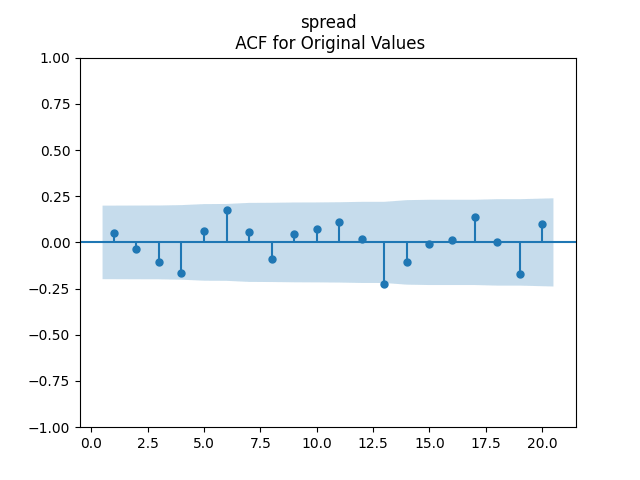
2-3. Then, modify the autoregression for log BAA rate to include spreads: This is vector autoregression of order 1:
It does NOT include volatility. It has intercept and the slope matrix
4. Model annual earnings by considering its growth: We model this as a regression
As usual, we fit it after dividing by volatility. We have
5. Next, we consider the bubble measure computed as in the above blog posts, with 10-year averaging window, and without using volatility. We get for and
This makes sense in the context of bond markets, even though we use geometric instead of arithmetic returns here. Note that this does not use volatility. Similar to the above post, we see:
7. Next, we fit the geometric Standard & Poor 500 returns by dividing it by volatility We also do regression versus
The quantity plays the role of the duration: Dependence upon the change in interest rates. This coefficient is negative because returns of stocks and bonds decrease when interest rates increase. Next, is the coefficient for the bubble measure. Of course, this is also negative, since being in a bubble implies low future returns. Same is true for the long-short spread, as discussed at the top of this post. Numerical values of coefficients are:
8. Finally, for international stocks we do the same. Thus we write this regression as
Note that is still the duration. Although is BAA rate, which is the USA, but it influences the international stocks as well. Same for the bubble measure. Numerical values of coefficients are:
Remark. In the regression for earnings growth, we tried instead of , but the p-value for the Student test is too large. Also, we tried instead of , but the p-value for the Student test is too large. We used covariates in linear regressions if Similarly, for the international stocks, we found that spread is not statistically significant.
Innovations. Thus we have 8 (eight) innovation series. Only for can be modeled as Gaussian. But all of them, judging by the autocorrelation function for and for and other tests, can be modeled as independent identically distributed random variables.
I do not have energy to present all these plots for each innovation series. But below is the table. Here, ACF is the L1 norm for the first 5 lags of the autocorrelation function values. Kurtosis is normalized so for normal distribution it is zero. Of course, the same is true for skewness.
Series
Length
Skewness
Kurtosis
Shapiro-Wilk p
Jarque-Bera p
ACF original values
ACF absolute values
Volatility
96
0.401
0.401
0.401
0.401
0.401
0.237
BAA rate
97
0.008
1.754
0.008
0.002
0.375
0.655
Long-short spread
97
1.058
3.382
0.000
0.000
0.455
0.468
Earnings growth
97
0.614
2.903
0.000
0.000
0.474
0.253
Bubble measure
97
-0.816
1.102
0.003
0.000
0.291
0.608
US corporate bond returns
52
0.193
0.238
0.857
0.800
0.878
0.706
US stock returns
97
0.039
0.157
0.344
0.940
0.413
0.590
International stock returns
55
-0.015
-0.202
0.941
0.953
0.527
0.331
Covariance matrix
Correlation matrix
See below the p-values for the Student T-test for null hypothesis which is zero correlation between series of innovations.
The main simulator gives users a choice of portfolio: US stocks, international stocks, and bonds. Moreover, the main choice in the portfolio is the proportion of stocks and bonds. In the newest version, we allowed this proportion to vary and not to be fixed throughout these simulated years. For example, at the start of 30 years, the stock/bond split can be 80/20, and at the end, 50/50. This is done to make room for retirement planning. Usually, people choose to invest more in risky assets at the start of their savings journey, and to make it less risky when they become closer to retirement. Within retirement, it is wise to do the converse: Invest in bonds less and less as you progress through the retirement.
Some users might be confused by this variability. In addition to options for withdrawals/contributions, this can be challenging to navigate. In practice, most users care about only a few modes: saving before retirement and living in retirement. To this end, I created a simplified version with the following options:
Risk Tolerance: High (Assertive), Mid (Moderate), Low (Conservative)
Your Goal:
Lump-Sum Investing: invest initial wealth, amount provided by user, and do not contribute annually
Regular Savings: start with zero wealth, contribute annually a fixed nominal amount, provided by user, which grows 3% annually
Retirement Spending: invest initial wealth, amount provided by user, and withdraw annually fixed nominal amount, initially it is 4% of the initial wealth, according to the celebrated 4% retirement rule, and grows 4% annually
Why choose 3% annual increase for annual contributions and 4% annual increase for annual withdrawals? Historically, inflation was running around 3% annually in 1928-2024. We consider only nominal (not inflation-adjusted) returns, because we could not model inflation-adjusted version of corporate bond returns. Thus we need some compensation for inflation.
Below, we provide the split between stocks and bonds: stocks/bonds. Stocks include both USA and international.
Lump-Sum Investing and Regular Savings:
Conservative: 60/40 constant during simulation
Moderate: 90/10 at the start, 60/40 at the end, linear during simulation
Assertive: 90/10 constant during simulation
Retirement Spending:
Conservative: 60/40 constant during simulation
Moderate: 60/40 at the start, 90/10 at the end, linear during simulation
Assertive: 90/10 constant during simulation
Other than that, in this simulator the user can choose the number of years, wealth (initial investment in case of lump-sum investing or retirement spending, or annual investment in case of regular savings), but not growth rate.


 at end of year
  paid at year
  and
and 
 as a simple autoregression of order 1 with trend:
  where
where 
 We fit
  The autoregression becomes the random walk (there is no mean-reversion) if
  but this hypothesis has
  which is very low. Next, the trend coefficient is zero if
  which has
 and compute the valuation measure
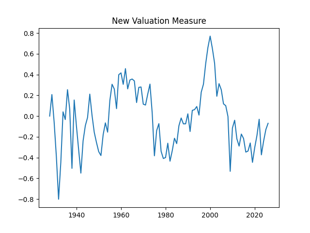
 as well as the quantile-quantile plot for
  The Shapiro-Wilk and the Jarque-Bera test give us
  and
and 
 as autoregression
 as another autoregression on the log scale
 as yet another autoregression
 as follows:
 Also the p-value for hypothesis
  is
is  The plots for residuals
  are below. This is independent identically distributed but not normal. Same is confirmed by the two normality tests, which give us extremely low p-values.
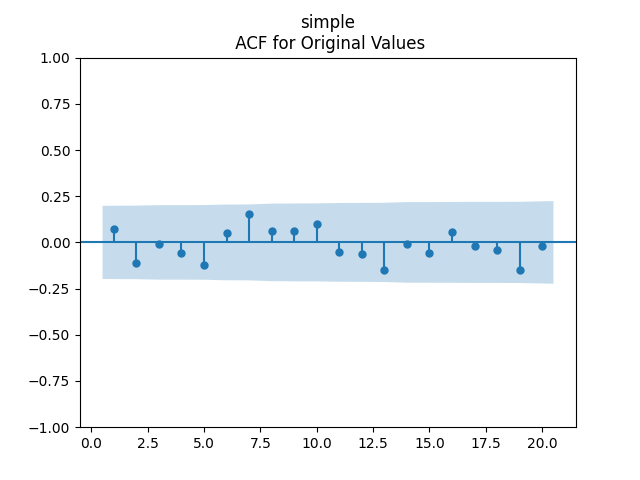
 regressed upon last year’s new valuation measure
  as yet another autoregression
 from the definition of the new valuation measure; and this does not have any new innovations. We modeled
  separately.
 The p-values are all
  or less. The normality tests for innovations
  can be modeled as independent identically distributed Gaussian, therefore; see the three plots below.
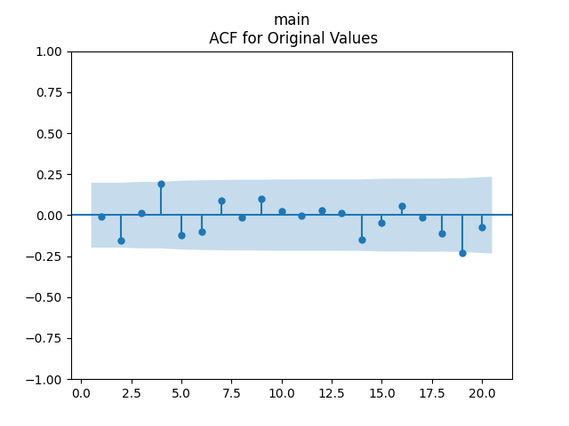
 in our time series models. Here
  is the BAA rate, December daily average for year
  The two other time series: the valuation measure
 is not significantly different from zero, with
  and the autocorrelation function and quantile-quantile plots for residuals
  shows this is not independent identically distributed and not Gaussian, see below.
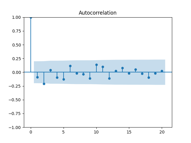
 instead of
  This means using rate itself instead of rate change as a factor. Or normalize this rate by volatility:
  In each case, still we have these plots as above for regression residuals.
 with p-values 8.6% for valuation coefficient zero and less than 0.1% for intercept and duration. Also, the residuals are Gaussian, with Shapiro-Wilk and Jarque-Bera normality tests giving us
  and
and  But not independent identically distributed. See the three graphs below.
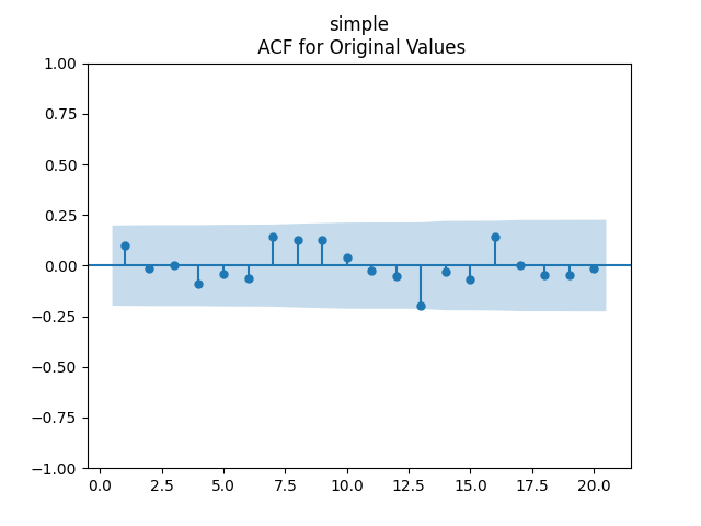

 with p-values 0.4% for valuation coefficient zero and 0.1% or less for others. Also, the residuals are Gaussian, with Shapiro-Wilk and Jarque-Bera normality tests giving us
  and
and  Finally, looking at autocorrelation function plots for
  we see that residuals are independent identically distributed Gaussian.
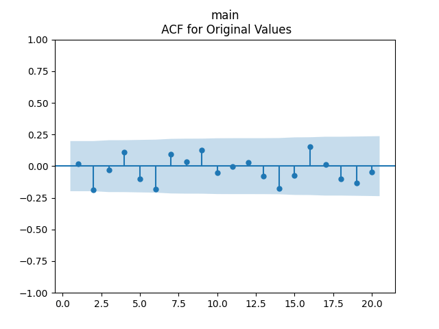
 annual realized volatility for the S&P for year
  for year
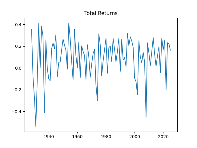
 And another autocorrelation function for their absolute values
  Both plots are below, and both are consistent with the white noise hypothesis. It is surprising that we, in fact, do not have to divide total returns by annual volatility to make it white noise.
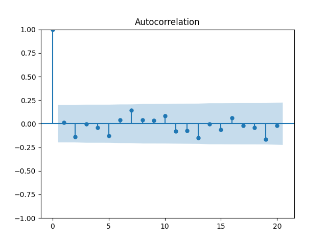
 and
and 
 Let us plot the autocorrelation function for
  and the autocorrelation function for
 for Shapiro-Wilk and Jarque-Bera normality tests.
 and
and  Also, plotting the autocorrelation function of
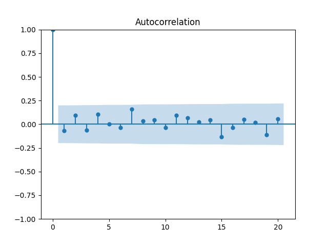
 are independent identically distributed. But it is more ambiguous to assume they are Gaussian, see the quantile-quantile plot below. The Shapiro-Wilk and Jarque-Bera tests give us
  and
and  respectively.
  We continue
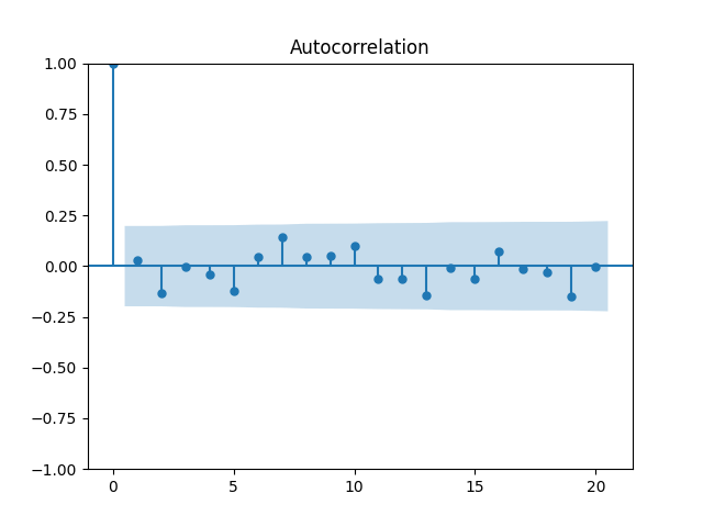
 and
and 
 and of
  and see that this is still consistent with being independent identically distributed. Only these values are slightly higher.
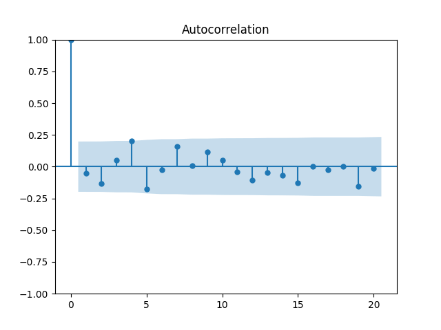
 and
and  respectively. See also the quantile-quantile plot. This is much closer to normal distribution.
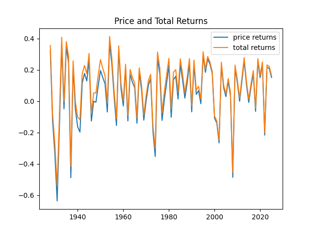

 and
and  But the p-value for the null hypothesis when we have a random walk is
  so we fail to reject the random walk hypothesis. This is not acceptable from the financial point of view, since the random walk implies
  will go negative eventually. Also, consider the graphs of autocorrelation function for
  These are not independent identically distributed.
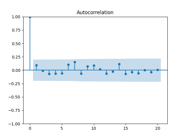

 and
and  with
with  for the null hypothesis of random walk, which corresponds to
  Plot the autocorrelation function for
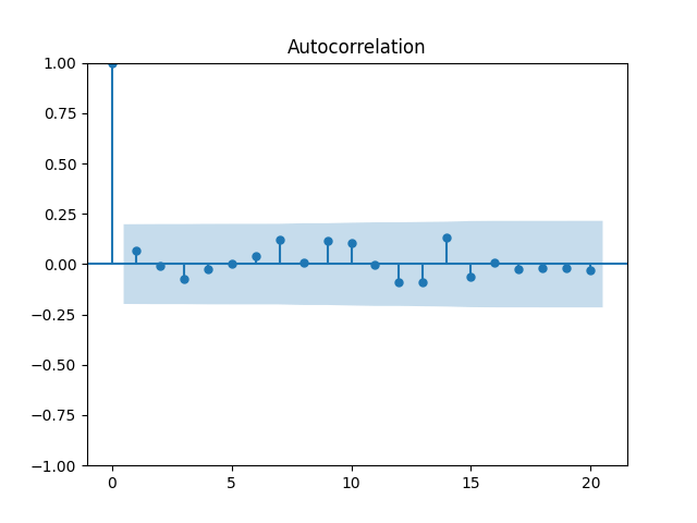

 are they really independent identically distributed Gaussian? Below are the autocorrelation function plots for
  and for
  which show that these are independent identically distributed.
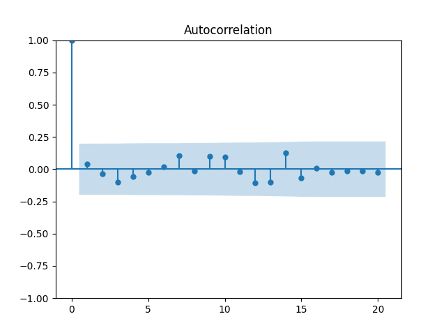
 and
and  which rejects the null hypothesis but are not as small as the previous ones.
  Below are autocorrelation function plots for
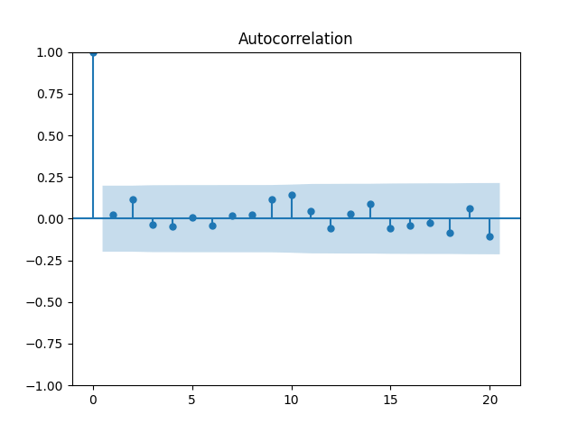
 and
and  This was done in the spirit of
  We continue
  which show lag 1, also the quantile-quantile plot.
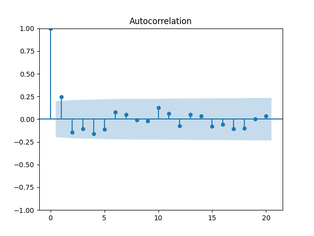
 and analyze it as well. The data are closer to the Gaussian distribution, with
  and
and 


 and
and  with
with  Shapiro-Wilk and Jarque-Bera normality tests give us
  and
and  See the graphs below, autocorrelation for
  autocorrelation for
  and the quantile-quantile plot for


 have changed:
 with
with  and
and  and
and 
 we have the density
 is the probability density function on
  for
for  which is the
  dimensional Gaussian distribution with mean vector
  and covariance matrix
  In other words, to simulate a random variable
  and simulate the additional noise
  independent of
  Thus
Thus 
 we apply Silverman’s rule of thumb: This is a diagonal matrix with
 are statistics of the
  th component of the data
  Namely,
  is the empirical standard deviation, and
  is the empirical inter quartile range: 75% quantile minus 25% quantile. This is realized in the file
  series of
  values. We then regress this last series (of course, only existing
  values) versus the full
  missing data points for series 3 (using series 1, 2, 4 as the backbone), and then to
  missing data points for series 5. We write this new data frame into a separate Excel file called filled.xlsx. It is available in
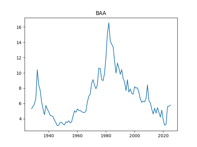


 This is vector autoregression of order 1:


 by considering its growth:
  We model this as a regression

 computed as in the above blog posts, with 10-year averaging window, and without using volatility. We get for
  and
and 


 by dividing it by volatility

 plays the role of the duration: Dependence upon the change in interest rates. This coefficient is negative because returns of stocks and bonds decrease when interest rates increase. Next,
  is the coefficient for the bubble measure. Of course, this is also negative, since being in a bubble implies low future returns. Same is true for the long-short spread, as discussed at the top of this post. Numerical values of coefficients are:

 is still the duration. Although
 instead of
  , but the p-value for the Student test is too large. Also, we tried
  Similarly, for the international stocks, we found that spread
  for
for  can be modeled as Gaussian. But all of them, judging by the autocorrelation function for
  and for
  and other tests, can be modeled as independent identically distributed random variables.


