Bond Returns 1973-2025

  1. Introduction and data description
  2. Relation between price returns and wealth process
  3. Fitting linear regression
  4. Conclusion

1. Introduction and data description. Continue the research after updating the data for 2025. In the previous post, we discussed total returns for S&P 500 in detail. Now we discuss bond returns. We take the same data as above, and for bond wealth process  B , we take FRED series BAMLCC0A0CMTRIV, last trading day of year 1972-2025. We start from  B(0) = 100 for the last trading day of 1972, and go on from there. This way we can compute log price returns for year  t.

2. Relation between price returns and wealth process. We derive log price returns from this wealth process using bond math. Then we run linear regression of this log price returns versus rate change. This regression coefficient is called the duration. In continuous setting, this is defined as minus derivative of the log price with respect to the interest rate. More precisely, we use yield to maturity as this interest rate.

Wealth at end of year  t-1 is  B(t-1) and at end of year  t is  B(t). Assuming the price of this bond at end of year  t-1 is  P(t-1) = B(t-1). Then the coupon paid during year  t is  B(t-1)R(t-1). The wealth at end of year  t is the sum of this coupon and the price  P(t) at end of year  t. Combining this, we get:  P(t) + B(t-1)R(t-1) = B(t).

We have  P(t)/P(t-1) = B(t)/B(t-1) - R(t-1). This gives us the formula for log price returns:

 Q(t) = \ln(P(t)/P(t-1)) = \ln(B(t)/B(t-1) - R(t-1)).

Since  B(t-1), B(t), R(t-1) are observed, we can compute  Q(t). If we fit this model, we can rewrite

 \ln(B(t)/B(t-1)) = \ln(\exp(Q(t)) + R(t-1)).

3. Fitting linear regression. As mentioned above, the log price returns  Q(t) can be regressed upon  -(R(t) - R(t-1)). We do not include an intercept into this regression, since this has the meaning of a discrete approximation of a derivative. The regression coefficient is 6.1053, and the residual analysis is done by the plots below. These are Gaussian but not quite independent identically distributed. This is confirmed by the p-values of Shapiro-Wilk and Jarque-Bera normality tests:  92\% and  75\%. And by the Ljung-Box test for 5 lags for original and absolute values of residuals, which give us  2.8\% and  4.3\%.

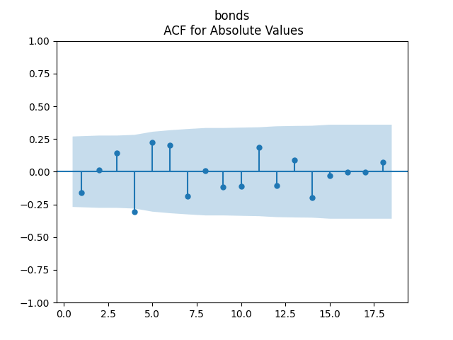
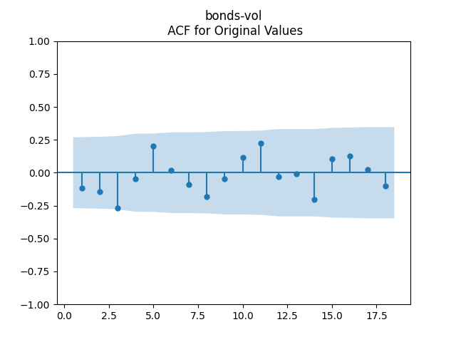
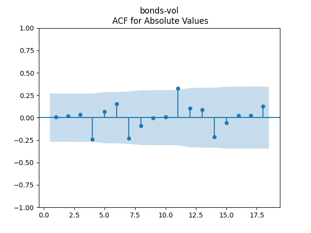
To make residuals independent identically distributed, we divide each term by annual volatility  V(t). This is equivalent to assuming that the residuals are heteroscedastic: These are white noise multiplied by  V(t). This gives us 5.96 regression coefficient, and  p = 86\% for Shapiro-Wilk normality test,  p =91\% for Jarque-Bera normality test. Also, the Ljung-Box test for the first 5 lags of original residuals has  p = 12\% and for absolute residuals has  p = 57\%. Finally, see the graphs for residuals below.

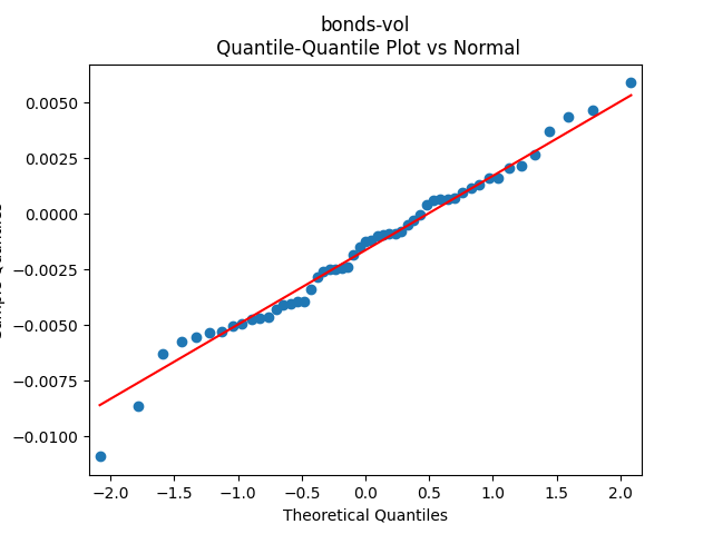
4. Conclusion. We have  \ln(B(t)/B(t-1) - R(t-1)) = -d(R(t) - R(t-1)) + Z(t)V(t) where  Z are independent identically distributed Gaussian. We succeeded in modeling the bond market! Duration in both cases is around  d = 6. What is more, this is better than previous models:

  • We clearly explain the meaning of duration as dependence measure of the price upon yield to maturity, and not rely on approximate formulas, such as in this blog post
  • We used volatility in our model, but stock volatility used for bond returns is highly unusual
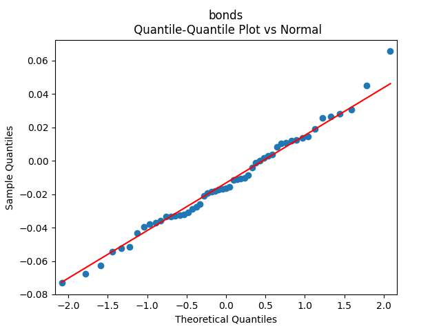
  • Residuals are independent identically distributed and Gaussian

Together with the two previous blog posts, we can now create a complete model of:

  • BAA rates
  • Dividends
  • The volatility
  • The valuation measure
  • Total stock returns
  • Total bond returns

These are 6 time series with 5 innovation sequences. Thus we can use it to create a simpler version of the financial simulator.

Published by


Leave a comment