My Finance

0. Introduction. Previously, we wrote a deterministic equation connecting the zero-coupon bond rates and the total returns for 10-year bonds. But we only approximated the zero-coupon bond rates with classic 10-year rates, for which we have much more data, back from 1927. And we need zero-coupon bonds to compute exact returns, not classic coupon Treasuries. Here, we explain and address this discrepancy.

1. Why we need zero-coupon bonds. Classic Treasury bonds pay semiannual coupons, so they pay 20 such coupons during their (for example) 10-year lifetime. We choose 10-year bond rates because they have the most data for them, going back to 1927 or even further. There are classic Treasury bonds with other maturities, for example 7-year or 30-year, but their data does not go back enough. Therefore, 10-year Treasury bond rates serve as the classic benchmark for long-term Treasury rates. They are free of default risk, but very much exposed to interest rate risk: If interest rates rise then bond prices fall. This is shown by duration, which is defined as the (minus) partial derivative of the price with respect to the rate. This can be thought of as average time of payments, weighted by the amount of payments (coupons and the principal). Thus we cannot exactly compute returns of such coupon bonds knowing only yield to maturity. We need to know the coupon rate, but usually only yield to maturity is quoted as the rate. This is a solution to a complicated equation which states that if we get coupons and reinvest them at the same rate, then the current price exactly matches all future payments. But this assumes the constant rate, which never happens.

The price (and therefore total returns) is much easier to compute for zero-coupon bonds, which pay only the principal amount. Their maturity, in fact, coincides with their duration. More precisely, if is end-of-year rate for the zero-coupon bond with maturity years and ith continuous compounding, then the price of this bond is One year later, at end of year this becomes a zero-coupon bond with maturity The new price is There are no coupons, therefore price and total returns coincide. The log returns are But where do we get these zero-coupon rates?

2. Data. Previously, it was not great with regard to zero-coupon bond rates data. We had Federal Reserve daily data from January 1990 until now, for maturities 1 year, 2 years, etc up to 10 years. But this is not nearly enough to make inference! Only 36 years. Instead, we found an article in Federal Reserve repository (their own internal version of arXiv or SSRN) which includes data from 1961 for zero-coupon maturities from 1 to 7 years and from 1971 for 8, 9, 10 years.

Target: We compute these log returns using these data for 9-year and 10-year end-of-year zero-coupon bonds, as in the subsection above.

Benchmark: But in addition, we replace and both by which is 10-year December average for year 10-year coupon Treasury rates. And we compute the new version of these log returns. See the GitHub repository where we put our newest version of the simulator with Gaussian innovations. We created a separate subfolder treasury-bonds with data and code files. The data file, as usual, contains detailed description.

We would use the target if we had data for zero-coupon bonds all the way from 1927. But unfortunately, we have them only from 1971. Which is a lot, but not enough. We approximate them by replacing them by the classic 10-year Treasury rate. But of course, this intorduces an error.

3. Analysis. How to compare these target and benchmark? The correlation is 97.7%. But this masks big differences, as shown in these data files. See the scatterplot and the time series plot below.

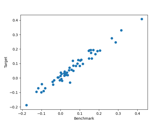
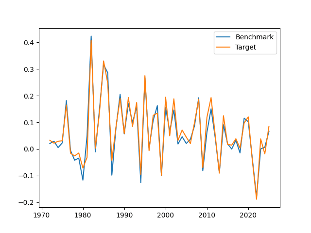
Run regression: Target = 0.954 * Benchmark + 0.01 + Residuals with But residuals are not Gaussian.

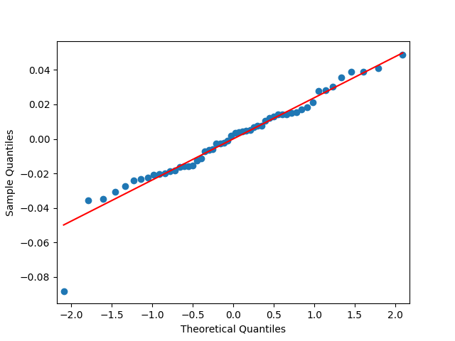
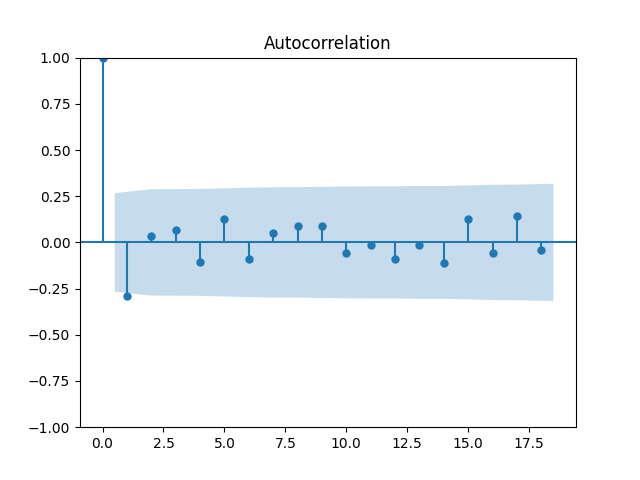
We tried dividing by volatility and thi did not work. Why such autocorrelation with lag 1? Because this difference is proportional to the long-short term spread (the slope of the Treasury yield curve), but this one has autocorrelation with lag 1, as shown in my current version of the financial simulator.

The Box-Cox transform works: Residuals become Gaussian, but still such a big autocorrelation. Still, lag 1 is the only one, so Ljung-Box white noise test for lags 5 and 10 gives us high p-values, so we fail to reject the IID null hypothesis. The Ljung-Box test for absolute values of residuals also gives us fail to reject.

4. Seven-year zero-coupon Treasury bonds. This turns out to be a better fit. For more years, 1962-2025 (64 years), not 1972-2026 (54 years), you can compute total returns. The above formula in Section 1 works for instead of The correlation is 97.3%, the linear regression is Target = 0.713 * Benchmark + 0.0205 + Residuals. And all tests above give p values above 5%. Thus we really can fit this regression. I will add these total returns for 7-year zero-coupon bonds into my main financial data library. See the Python file in the same subfolder treasury-bonds. We do not need the Box-Cox transform, after all.