My Finance

Introduction: Continuing the previous post, we consider the analysis for the value-based portfolios. We take total and price arithmetic annual returns for 1927-2025 for cap-weighted portfolios. The same GitHub repository stores the data and code. Again, we repeat this analysis. We also regress the next year’s total log returns vs this year’s new valuation measure.

Methodology: We shall not repeat the methodology here in this post. Recall only that

The trend is and we consider the vlauation measure as

Unlike in the previous post, we rank stocks not by size (market capitalization), but by the book yield: the ratio of book value to market value. We consider 30%/40%/30% split, also quintiles and deciles.

Failures: We could not even compute for the top 9 and 10 deciles. This stands in contrast from the size-based portfolios, where we failed to compute it for the bottom 1 decile. In both cases, the failure was due to the fact that total and price returns coincide for some years, and therefore the dividend paid is zero, so we cannot take its logarithm. Similarly, we could not compute it for the top quintile. This is surprising, and we do not know how to explain it. In fact, stocks with high book yield ratios are likely to have high dividends, not zero dividends. Below, we consider results for the deciles 1-8.

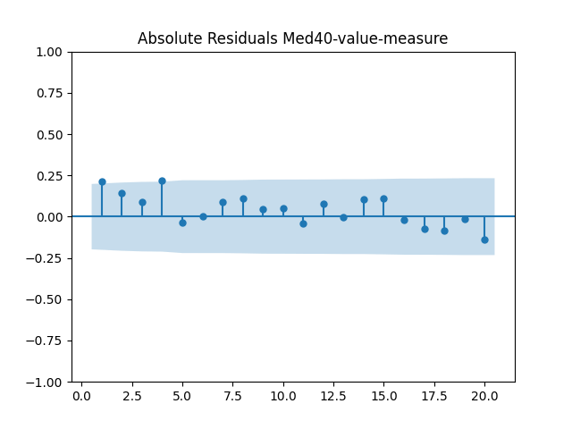
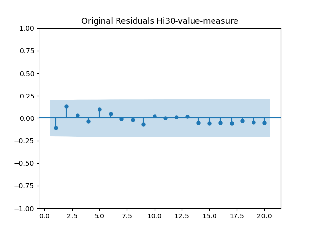
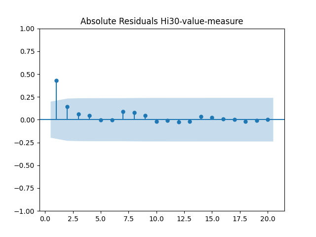
Results: The trend number is around 4%-5%. This again suggests that this trend is a fundamental constant, similar to other cases. Again, we discussed it in my previous blog post. See also my article which has extensive discussion about this. We see, surprisingly, that we reject the independent identically distributed hypothesis for residuals for deciels 7 and 8. What is wrong with these value stocks with high book yields? Finally, the random walk hypothesis that is always rejected.

Decile	Trend	RW	LB-orig	LB-abs
1	4%	0.8%	32%	38%
2	4.7%	0.2%	62%	32%
3	5%	0.1%	45%	29%
4	5%	0.0%	4.5%	24%
5	5.3%	0.2%	14%	95%
6	5.1%	0.7%	25%	45%
7	5.2%	0.5%	0.3%	2%
8	5.3%	0.0%	24%	0.0%

We also mention that both Shapiro-Wilk and Jarque-Bera normality tests show normal residuals for Deciles 1-3.

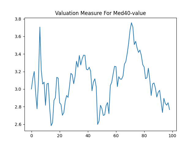
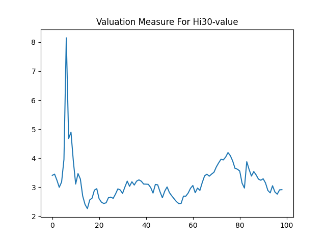
Measure Plots for Low 30%/Mid 40%/High 30%: Let us plot the autocorrelation function for and for as well as the valuation measure for each of these three portfolios. We see that growth stocks (low 30%) and blend stocks (middle 40%) are showing bubble in the 1960s and the 1990s. But value stocks (top 30%) show the bubble in the 1930s but not so much in the 1990s (only a bit).

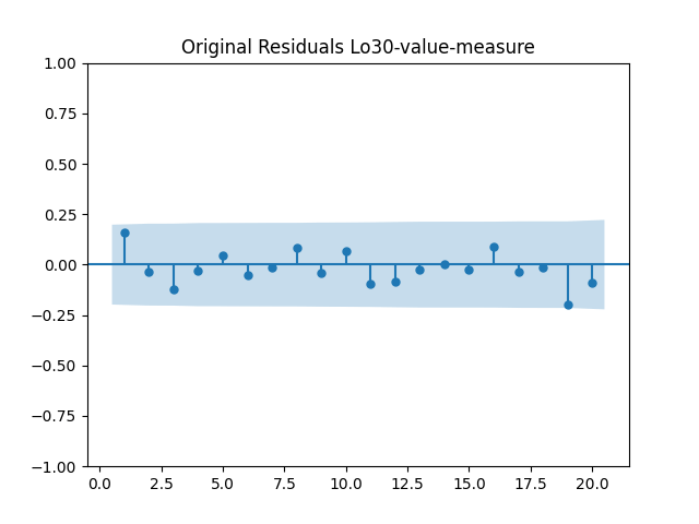
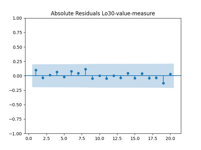
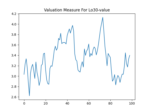
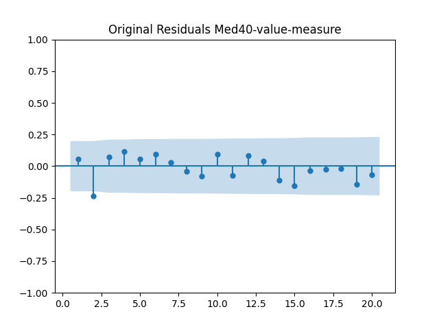
Returns vs measure: Now regress the total log returns vs last year’s new valuation measure Namely, fit

Below we show the table for the 8 deciles, giving the slope and the intercept as well as the value for the Student T-test. Interesting results! For the bottom 5 deciles, we have almost the same slope and intercept, and we reject, or almost reject, zero correlation. But for deciles 6-8, we have almost zero slope, and we fail to reject the zero correlation hypothesis. Again, I do not understand why we have this!

Decile	Slope	Intercept	Student Test
1	0.14	0.59	0.9%
2	0.14	0.55	1.5%
3	0.13	0.50	6.7%
4	0.14	0.54	6.9%
5	0.15	0.56	6.4%
6	0.02	0.18	78%
7	0.06	0.27	39%
8	0.03	0.22	37%

Now try analyze for independent identically distributed Gaussian. Judging by the Shapiro-Wilk test, we always reject normality. But Jarque-Bera test gives us rejection only for deciles 4-8. Again, I do not understand why this is so. For the Ljung-Box test, we never reject white noise for original residuals, but we reject this for absolute residuals if we have some deciles. Only for smallest deciles (growth stocks) we have IID Gaussian. Why??

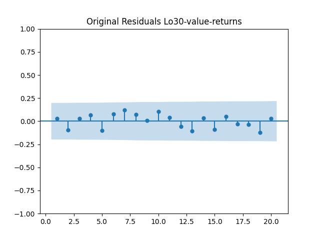
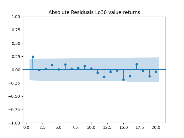
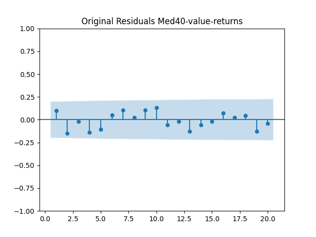
Returns Plots for Low 30%/Mid 40%/High 30%: Try plotting residuals autocorrelation functions for and for low 30% (growth stocks), mid 40% (blend stocks), and high 30% (value stocks). We see that we have problems with but not so much with But autocorrelations are away from zero mostly for lags 1 and 2. I think this supports using the stochastic volatility much in the same way as in previous posts.

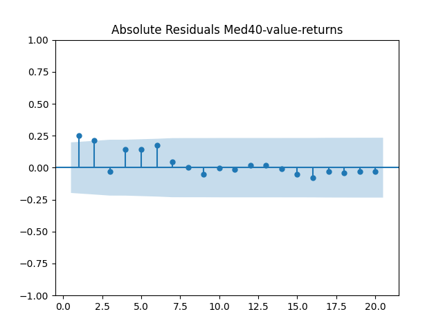
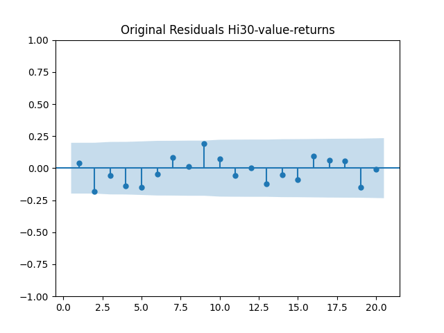
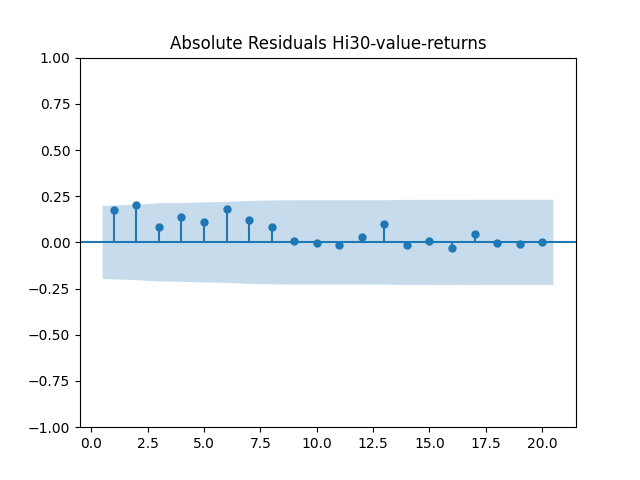
Conclusion: And we can reproduce some of the bubble analysis using our new dividend-based valuation measure. But still, there are many enigmas here. We must consider stochastic volatility. First use the overall S&P volatility, then the volatility for daily returns of each such portfolio, which is also available from the same Data Library.

This is the 64th post in my blog!! Hooray!