Introduction: We recomputed the new dividend-based valuation measure discussed in the previous posts for the Fama-French size-based portfolios (cap-weighted, annual returns, 1928-2025) taken from their data library. We consider total returns and price returns. They are arithmetic but they can be converted into geometric. And from there, one can compute dividends paid. The code and data are available on GitHub. We updated the code, the previous version contained mistakes.
Dividend-Based New Valuation Measure: We consider the difference between total log returns and log dividend growth and denote it by 

We analyze the residuals 
Results for Ten Deciles: Mostly (except the most small stocks), the residuals are IID (both the ACF of original values and the ACF of absolute values correspond to white noise). But usually, except for the largest portfolios, they are not Gaussian. Always, all coefficients 


In the table below, SW p and JB p stand for Shapiro-Wilk and Jarque-Bera normality tests p-values, LB-orig and LB-abs stand for the p-values of the Ljung-Box test for white noise for 5 lags if we take original and absolute values of residuals; 
| Decile | SW p | JB p | LB-orig | LB-abs | R squared | RW p | Trend |
| Smallest 10% | N/A | N/A | N/A | N/A | N/A | N/A | N/A |
| Decile 2 | 0.00% | 0.00% | 0.11% | 0.04% | 22.5% | 0.0% | 3.7% |
| Decile 3 | 0.00% | 0.00% | 93% | 0.1% | 9.4% | 0.2% | 4.5% |
| Decile 4 | 16% | 2.4% | 96% | 44% | 7% | 1% | 4.7% |
| Decile 5 | 0.82% | 0.01% | 1.73% | 5% | 6.7% | 1.4% | 4.8% |
| Decile 6 | 5.4% | 0.02% | 36% | 44% | 7.4% | 0.8% | 4.91% |
| Decile 7 | 4.2% | 15% | 70% | 65% | 8.9% | 0.4% | 4.96% |
| Decile 8 | 49% | 51% | 95% | 54% | 7.6% | 0.7% | 5.06% |
| Decile 9 | 28% | 18% | 68% | 69% | 8.8% | 0.4% | 4.99% |
| Largest 10% | 86% | 59% | 46% | 73% | 6.4% | 1.2% | 4.94% |
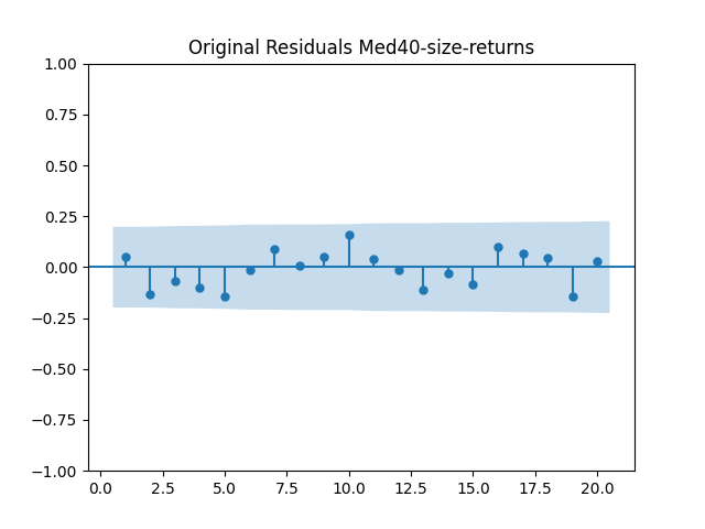
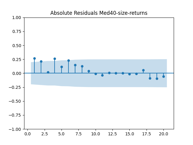
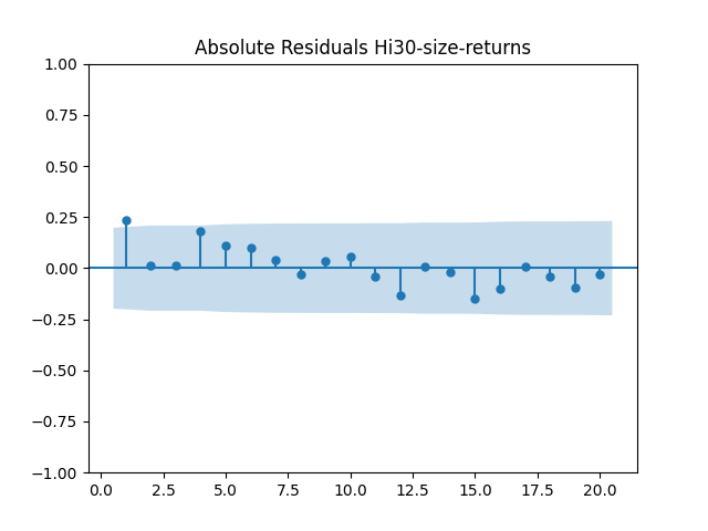
Three Size-Based Portfolios: We also did analysis for lower 30%, middle 40%, largest 30%, and the five quintiles, but we do not present them in this table. Let us instead present ACF plots for original and absolute values, and the valuation measure for these.
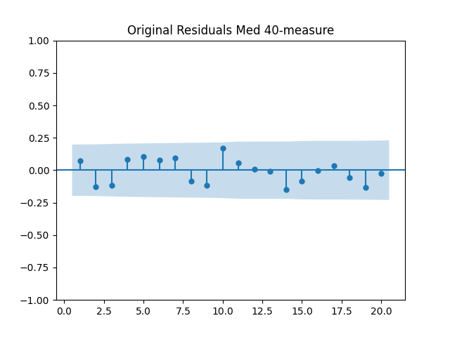
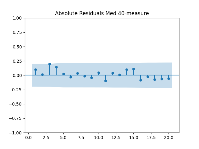
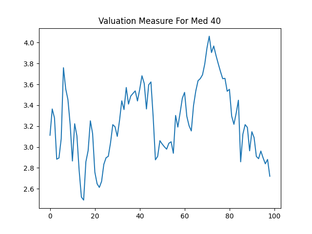


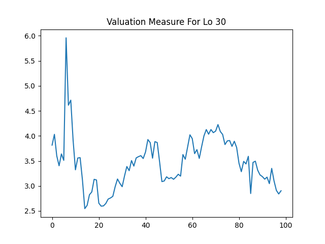

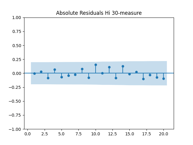
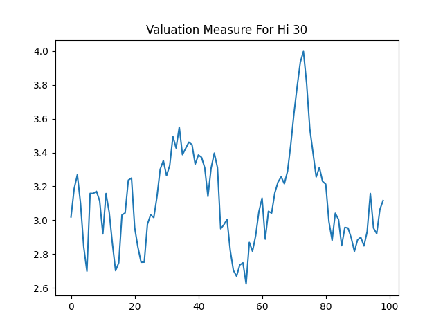
We see that the valuation measure looks very different for low 30% stocks vs mid 40% and high 30% stocks. We see a huge bubble in small stocks during the Great Depression but there is not much bubble during the late 1990s. For contrast, the medium stocks show both bubbles, as well as the bubble in the 1960s. And the large stocks show especially large bubble during the dotcom era. But the autocorrelation function plots are consistent with independent identically distributed assumption.
Total Returns vs Valuation Measure: Let us regress next year’s total log returns 


See below the autocorrelation function plots for 

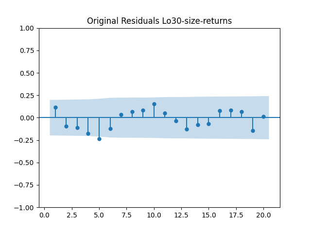
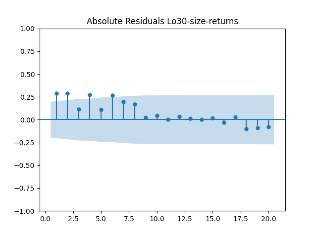

But what about 


Judging by the Shapiro-Wilk normality test, we always reject normality.
Conclusion: Imagine the possibilities: Now given the price and total returns, we can compute the entire new valuation measure and its influence upon the next year’s total returns. But we did not include annual volatility. But maybe we should! Such volatility is also available from the Kenneth French’s data library. Indeed, we can compute it from daily returns. This opens rich possibilities for further analysis.
See the next blog post for analysis of value-based portfolios.


Leave a Reply