My Finance

1. Motivation of the new valuation measure
2. Fit autoregression with linear trend as before
3. Use this valuation measure for modeling returns
4. Include bond rates and duration
5. Conclusion

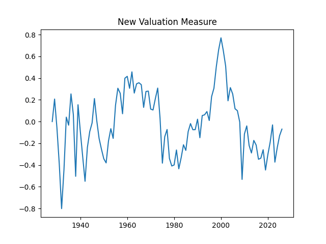
1. Motivation of the new valuation measure. We continue the previous blog post. We replicate the valuation measure here. We use updated data for 2025. Previously we did this with 10-year earnings but now we wish to do this with 1-year dividends.

We prefer dividends to earnings for the following reasons:

• Dividends are the actual cash paid, and they are not disputable, but earnings depend on accounting standards
• Dividends are more predictable, since companies do not like to cut them, but earnings are highly volatile
• Earnings of companies can be negative, and thus suffer from the aggregation bias, but dividends are nonnegative

2. Fit autoregression with linear trend as before: Take the index level at end of year and dividends paid at year Total returns and dividend growth are given by and

We model the cumulative difference as a simple autoregression of order 1 with trend: where are innovations. The valuation measure then is defined as

This can be written as We fit The autoregression becomes the random walk (there is no mean-reversion) if but this hypothesis has which is very low. Next, the trend coefficient is zero if which has

From here, we can deduce and compute the valuation measure The measure, as before, shows us that the market is not overvalued, since it is average compared to the historical standard.

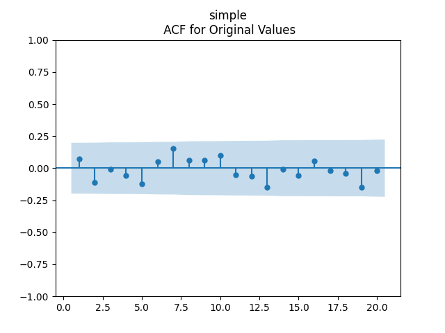
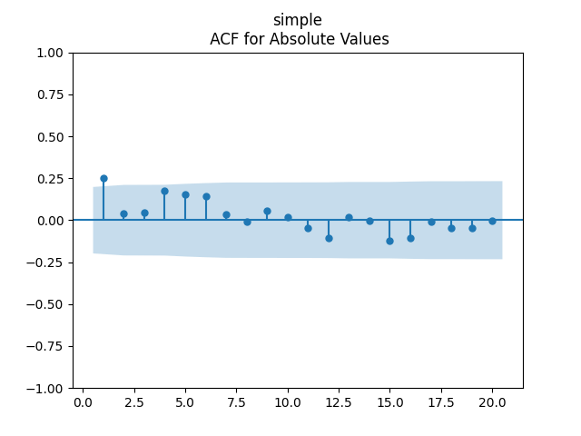
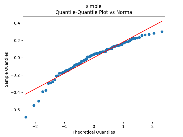
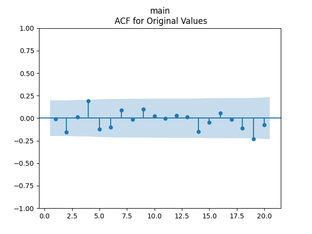
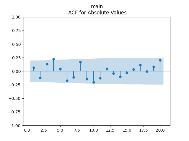
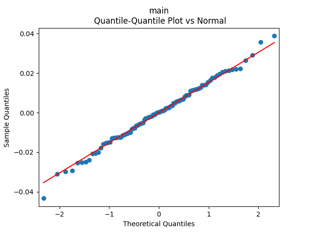
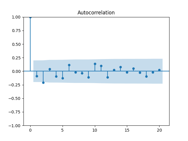
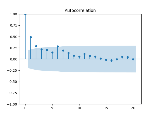
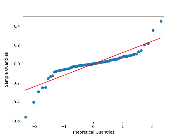
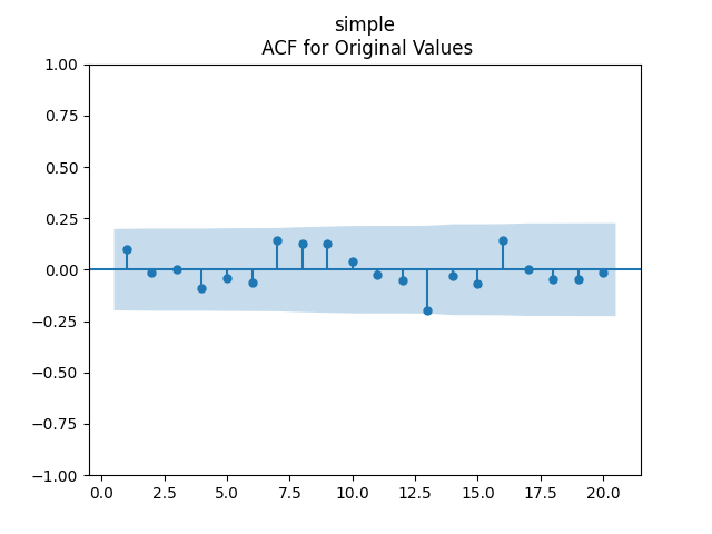
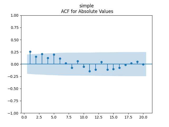
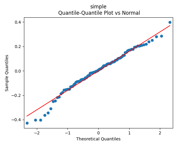
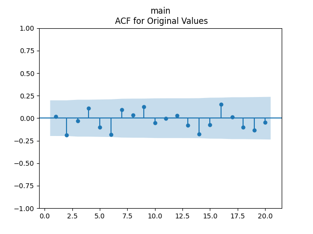
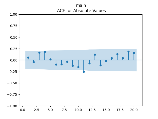
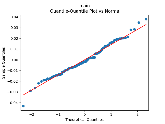
Analysis of residuals: See the autocorrelation function plots for and for as well as the quantile-quantile plot for The Shapiro-Wilk and the Jarque-Bera test give us and

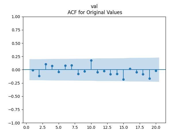
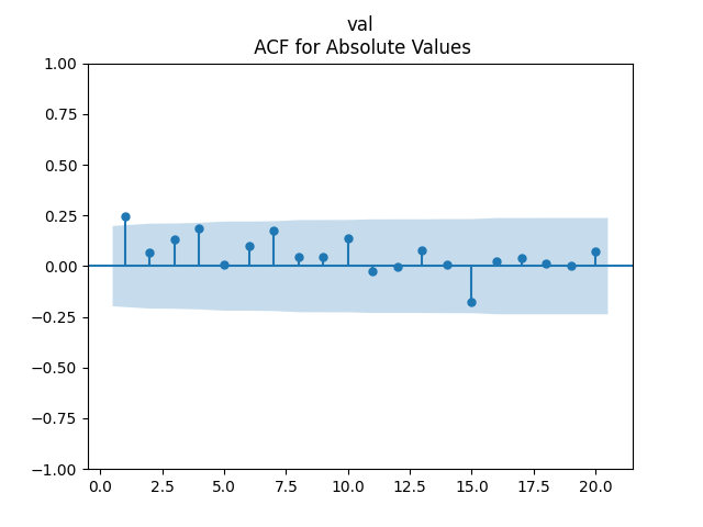
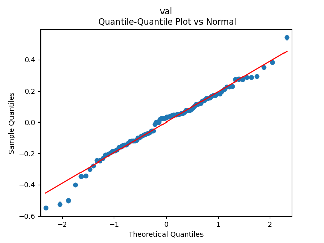
We can approximately assume that residuals are independent identically distributed Gaussian, although the autocorrelation function for lag 1 for the absolute values of innovations raises questions.

3. Use this valuation measure for modeling returns. We can model total stock returns with dividends.

Model 1. Since we know how to model dividend growth from the previous blog post, together with annual volatility, we can simply model stock returns using three time series:

• the new valuation measure as autoregression
• volatility as another autoregression on the log scale
• normalized dividend growth as yet another autoregression

Model 2. However, we can also regress upon as follows:

We get Also the p-value for hypothesis is The plots for residuals are below. This is independent identically distributed but not normal. Same is confirmed by the two normality tests, which give us extremely low p-values.

This model uses four time series, but with only three series of innovations:

• returns regressed upon last year’s new valuation measure
• the new valuation measure as the detrended difference of total returns and dividend growth
• volatility as another autoregression on the log scale
• normalized dividend growth as yet another autoregression

The second time series is without new innovations: Indeed, we simply write from the definition of the new valuation measure; and this does not have any new innovations. We modeled and separately.

Model 3. Let us modify Model 2 to include division by volatility: We divide by both returns and the right-hand side.

We get The p-values are all or less. The normality tests for innovations show p-values above 90% and this is confirmed by the plot below. The values of can be modeled as independent identically distributed Gaussian, therefore; see the three plots below.

This model also uses four time series but with three series of innovations, as in Model 2.

4. Include bond rates and duration. Following the previous blog post, we include rate change in our time series models. Here is the BAA rate, December daily average for year

Model 1. Try to include this rate change as a factor in dividend growth model The two other time series: the valuation measure and the volatility do not need rate change as the factor. We get:

But we run into problems: The coefficient is not significantly different from zero, with and the autocorrelation function and quantile-quantile plots for residuals shows this is not independent identically distributed and not Gaussian, see below.

Similar results are if is divided by Thus we abandon this idea of including duration (dependence upon rate change) in normalized log dividend growth.

Finally, try to include instead of This means using rate itself instead of rate change as a factor. Or normalize this rate by volatility: In each case, still we have these plots as above for regression residuals.

Conclusion: We failed to model normalized dividend growth using rate or rate change for BAA bonds.

Model 2. Include duration in the regression for total returns, together with the valuation measure:

We get with p-values 8.6% for valuation coefficient zero and less than 0.1% for intercept and duration. Also, the residuals are Gaussian, with Shapiro-Wilk and Jarque-Bera normality tests giving us and But not independent identically distributed. See the three graphs below.

Conclusion: We failed to include duration in total returns modeling without normalizing by volatility.

Model 3. Include duration in the regression for total returns, together with the valuation measure:

We get a much better fit than without the duration or in Model 2: with p-values 0.4% for valuation coefficient zero and 0.1% or less for others. Also, the residuals are Gaussian, with Shapiro-Wilk and Jarque-Bera normality tests giving us and Finally, looking at autocorrelation function plots for and for we see that residuals are independent identically distributed Gaussian.

Conclusion: Here we succeeded in including the duration as a factor for regression modeling of total returns after normalizing.

5. Conclusion: We can reasonably model the new valuation measure using one-year dividends, not trailing ten- or five-year earnings, as in previous articles or blog posts. This might be better, since in previous models we used both dividends and earnings, but here we use only dividends. It is useful to include rate change as a factor in a regression for total returns, but only after normalizing, and not for normalized dividend growth. This updates our blog post. In the next post, we consider total corporate bond returns modeling using bond rates.