See my GitHub repository simulator-current for the HTML frontend pages, Python backend code in Flask, Excel data file, and Python code for validation of the model described below.
Continuing the previous post, we updated the financial simulator to make for geometric returns instead of arithmetic returns. We had mistakenly made linear regression for arithmetic returns, but this does not work well, since such returns can be only greater than 
- Description and system of equations.
- Testing innovations for white noise.
- Testing innovations for normality.
Description and system of equations
We use the following autoregression equation for annual volatility for S&P 500 and its predecessor, S&P 90, computed by Angel Piotrowski:


Next, we use the following autoregression for BAA rate, following previous research:


We use the logarithm because otherwise the rate might become negative, even with very small probability.
We consider three classes of assets and denote their annual geometric total returns (multiplied by 100 for normalization):
- USA stocks, measured by Standard & Poor 500 index and its predecessor, the Standard & Poor 90 index
- International stocks, measured by MSCI EAFE (Europe/Australasia/Far East) index
- USA corporate investment-grade bonds, measured by Bank of America ICE index (ratings AAA, AA, A, BBB)


We normalize the two stock returns by dividing them by annual volatility. But we do not normalize the bond returns. We have the following equations for these three classes of assets:
- For USA corporate bonds, following this blog post, we get:
with
and
- For USA stocks, following this blog post, we get:
with
and
and
- For international stocks, similarly to USA stocks, we get:
with
and
and


Thus all three classes of assets have returns highly dependent upon change in interest rates, with duration (regression coefficient) 


All five series of residuals 
Unfortunately, they are not normal. Namely, 


However, I still modeled these five series as multivariate Gaussian with mean vector zero and the following empirical covariance matrix.

We consider only nominal, not real returns. To compensate for that, withdrawals/contributions can change annually.
We allow for constant split between US and international stocks. Bond and overall stock percentages might change from year to year linearly. This is to allow for a more conservative portfolio as time goes.
Also, and very importantly, we added a separate web page with a simplified version of this simulator. We describe it in a separate post.
Initial value for volatility is taken as average daily close VIX June 1, 2024 – May 31, 2025. The initial value for the BAA rate is taken as average daily May 2025.
Testing innovations for white noise
Below are autocorrelation function plots for the five series of innovations. Original and absolute in the captions refer to whether innovations are taken as is or after taking absolute values.
has tag ln-vol
has tag ln-baa
has tag bonds
has tag usa-stocks
has tag intl-stocks
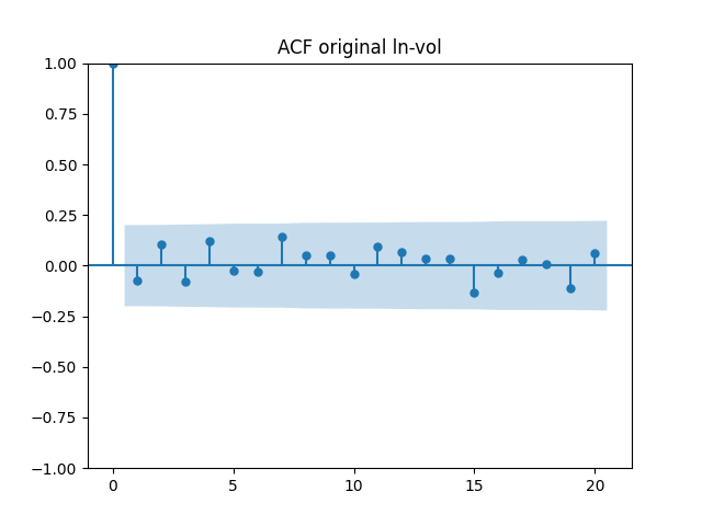
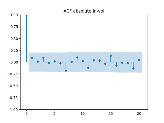

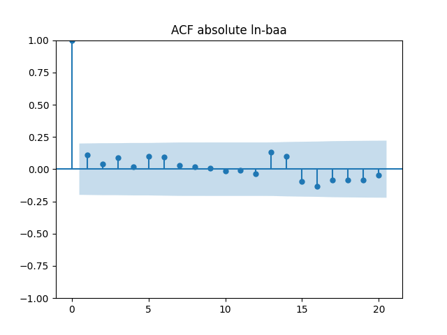
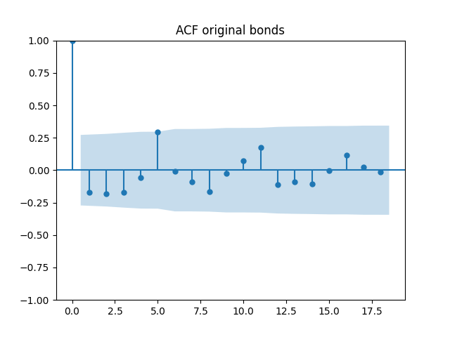
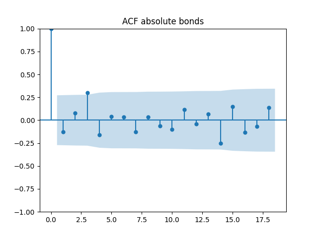
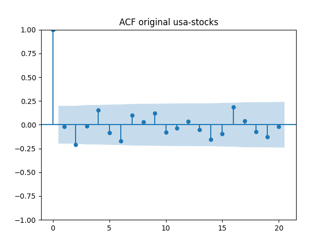
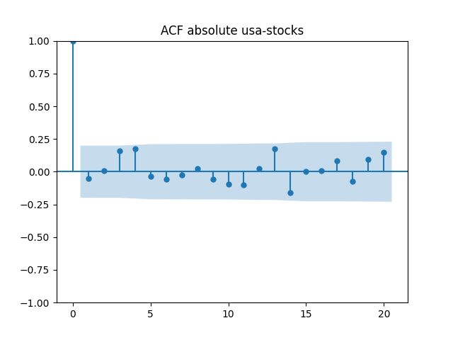
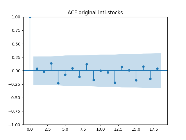
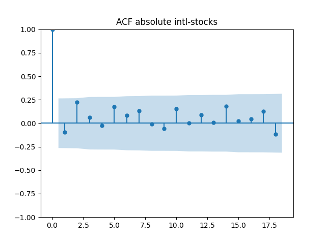
Also, we compute L1 norms for first 5 values of the ACF, for original innovations and their absolute values. Comparing with these threshold values, we see that it is reasonable to model these as independent identically distributed.
| N Data Points | 96 | 97 | 52 | 97 | 55 |
| Innovations | | | | | |
Original  | 0.40 | 0.18 | 0.88 | 0.48 | 0.49 |
Absolute  | 0.24 | 0.36 | 0.71 | 0.43 | 0.58 |
Testing innovations for normality
Similarly, we plot the five quantile-quantile plots versus the normal distribution below. Tags are the same.
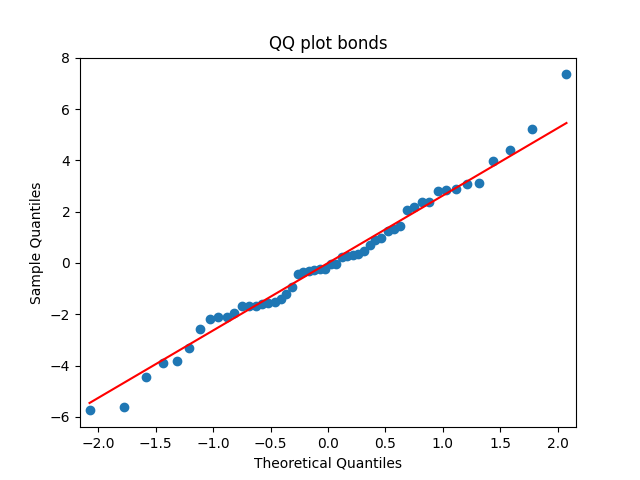
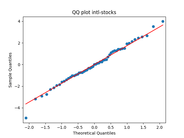
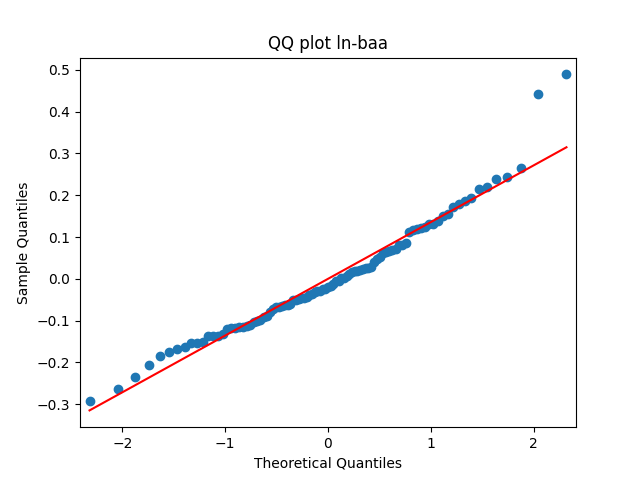
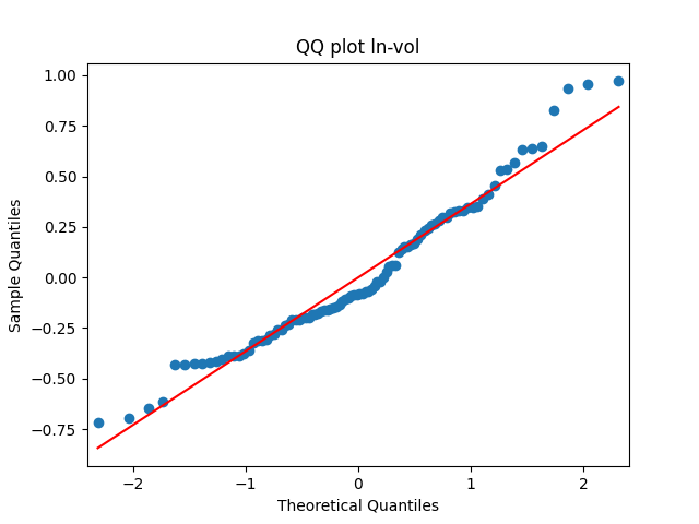
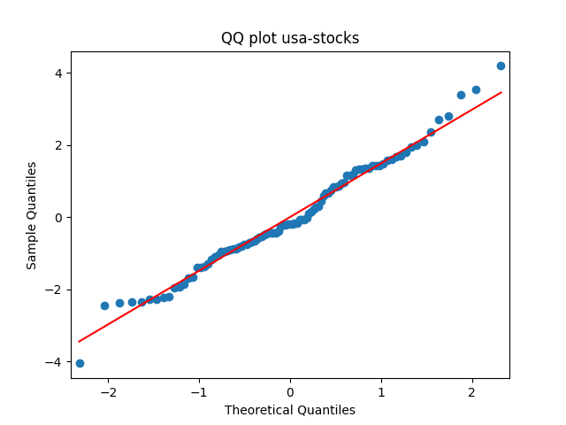
Also, see p-values for statistical testing for normality: Shapiro-Wilk (SW) and Jarque-Bera (JB) testing.
| Test | | | | | |
| SW | 0.9% | 0.6% | 86% | 42% | 99% |
| JB | 6.1% | 0.009% | 80% | 66% | 90% |
Finally, let us provide skewness and kurtosis for these innovations, normalized so that for the normal distribution they are 0.
| Function | | | | | |
| Skewness | 0.59 | 0.81 | 0.19 | 0.23 | -0.13 |
| Kurtosis | 0.057 | 1.4 | 0.24 | 0.068 | 0.13 |
Summary: 

Leave a reply to Bubble Measure and Long-Short Spread in the Simulator – My Finance Cancel reply