My Finance

We continue part III of the blog post. There, we modeled price and total returns of S&P 500 (both nominal and real) as a linear regression with four factors: three bond spreads BAA-AAA, AAA-Long, and Long-Short; and earnings yield (last year’s earnings divided by the end-of-year index level). Look at that blog post for background and definitions.

As usual, we had regression residuals multiplied by annual volatility. Also, as usual, we added this volatility as the fifth factor. So that after dividing the regression equation by this volatility and applying ordinary least squares fit, we still have an intercept in this new regression equation.

Here, we change this classic earnings yield to its cyclically adjusted version. We allow any averaging window between 1 and 10 years.

We make another change compared to the blog post: Instead of the earnings yield as a factor in linear regression for total/price and nominal/real returns, we take the logarithm of this earnings yield. This is motivated by a remark at the end of this post.

We also add results of parts I and II in the blog post and unite them in the same Python code file. This is different from the blog post, where we split the Python code in 3 files corresponding to each part I, II, III. The code and data are on GitHub/asarantsev repository 3spreads-CAPE-simulator

Consider the linear regression

Here, are spreads: BAA-AAA, AAA-Long, Long-Short, and cyclically adjusted earnings yield (average earnings over the last few years divided by end-of-year stock index. As usual, is annual realized inflation, and are independent identically distributed. We fit this for windows of 5 and 10 years, and for which are total/price returns, real/nominal versions.

Methods: We apply standard analysis of residuals , outlined in this previous post. We also consider of this regression and compare this with cut version without any spreads. Finally, we consider the Student T-test for each coefficient.

Results: All residuals can be reasonably modeled as IID Gaussian. All coefficients in the large regression are NOT significant. The most significant (having smallest p-value) among spreads is usually BAA-AAA. Adjusted does not change much for price returns and barely for total returns.

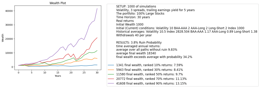
Conclusion: This is a great model. We can use it in the simulator, which we uploaded in https://github.com/asarantsev/3spreads-CAPE-simulator

Simulation: We allowed to change the index level, three spreads, and volatility for the initial conditions. But we did not allow to change trailing annual earnings. We have an entire averaging window, we do need this, as shown in the previous research. Input of 5 or 10 annual earnings would be cumbersome for a user. However, input of current price is easy.

Also, it’s easy to look for current S&P 500 level, rates (which lead to spreads) and volatility (measured by VIX) in the market. But it’s harder to look up last few years of earnings. Anyway, these earnings change slowly and are updated rarely.