My Finance

This is a big post (the biggest on blog so far) which extends our previous posts:

• Four bond rates from 1927
• S&P 500 Returns using Earnings Yield and Volatility
• Dividing annual earning growth by volatility makes them Gaussian white noise
• Vector autoregression with volatility for two spreads
• Growth/Volatility vs Spreads
• Stock Returns vs Earnings Yield and Two Spreads
• Make S&P Returns IID Gaussian
• Does dividing by volatility improve fit for bond spread?

The data is available on my personal web page. The code is available on my GitHub/asarantsev repository 3spreads-1yearnyield-returns which contains 3 Python code files corresponding to 3 parts of this post:

• PART 1. Modeling bond spreads BAA-AAA, AAA-Long, Long-Short as vector autoregression
• PART 2. Modeling earnings growth using these bond spreads as regression factors
• PART 3. Modeling S&P returns using 1-year earnings yield and these bond spreads as regression factors

PART 1: Modeling bond spreads BAA-AAA, AAA-Long, Long-Short using vector autoregression of order 1, with innovations normalized by annual volatility. This model fits well and is stable in the long run, with IID but not quite Gaussian innovations.

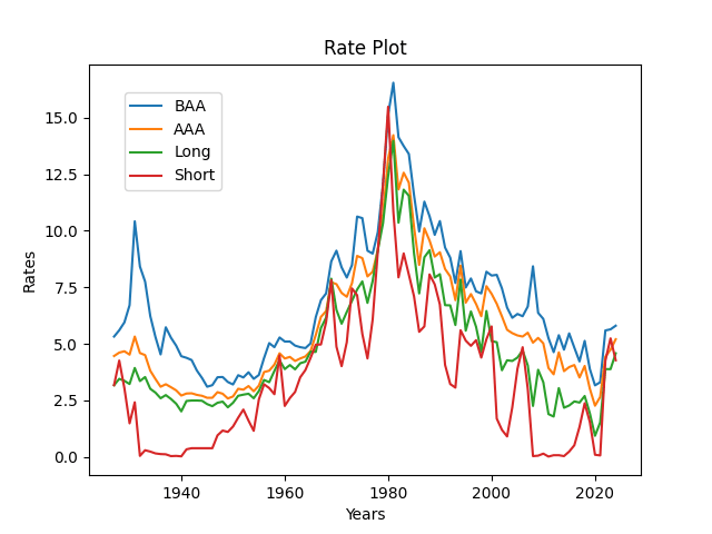
Data: We consider four bond rates, average daily December data 1927-2024, at end of year t:

1. Long stands for 10-year Treasury rate (1963-now), long-term government securities (1927-1962)
2. Short stands for 3-month Treasury rate (1934-properly extended to earlier data), and short-term (3- and 6-months) government securities (1927-1933)
3. BAA is Moody’s rates for portfolios of investment-grade corporate bonds with BAA ratings (1927-2024)
4. AAA is Moody’s rates for portfolios of investment-grade corporate bonds with AAA ratings (1927-2024)
5. Annual realized volatility of Standard & Poor 90/500 (1928-2024) daily log returns for year

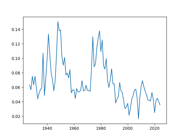
See the time graph of interest rates below. This continues research from the previous blog post.

Next, we take three bond spreads: BAA-AAA, AAA-Long, Long-Short. See the time graph below.

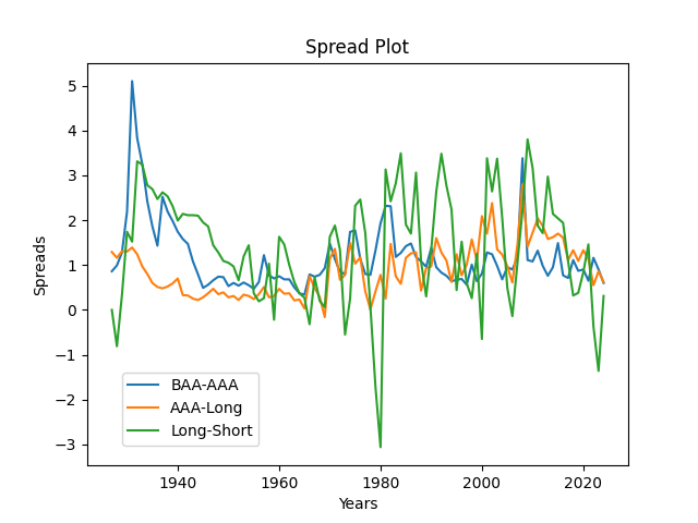
Model: Consider the vector S(t) of three bond spreads. We model it as where and is a 3\times 3 matrix, and is a sequence of independent identically distributed (IID) trivariate random vectors with mean zero. This is an extension of the same model for two spreads: BAA-AAA and AAA-Long, which, in turn, continues this research.

As usual, we also have log Heston model for the volatility: where are IID with mean zero. We already fit it in the previous post, so we do not discuss it here.

We fit this multivariate model for by each of three scalar equations. We divide this equation by the volatility and then use ordinary least squares method. Then we test each of the three components of the innovation series for IID Gaussian using the usual procedure:

1. Empirical skewness and kurtosis (both = 0 for Gaussian)
2. Shapiro-Wilk and Jarque-Bera normality tests p-values
3. L1 norm for the autocorrelation function for lags 1, \ldots, 5, of and
4. Autocorrelation function plots for and for
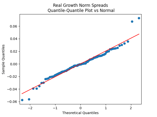
5. The quantile-quantile plot of versus the normal distribution

Results for coefficients: We have the following point estimates:

The Student T-test gives us only for diagonal values of B, its third row, and c. It is important to verify that eigenvalues of B are strictly less than 1. Then the time series model above is stable and ergodic in the long-run, see my manuscript arXiv:2411.03699: Zero-Coupon Treasury Rates and Returns using the Volatility Index with Jihyun Park. It has a unique stationary distribution, see this work. But this is left for further research.

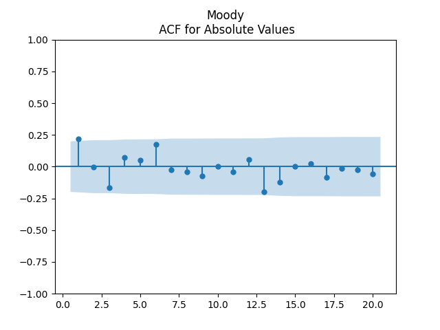
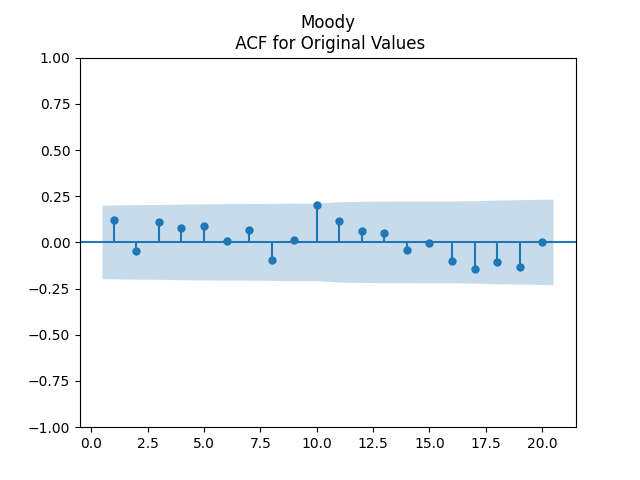
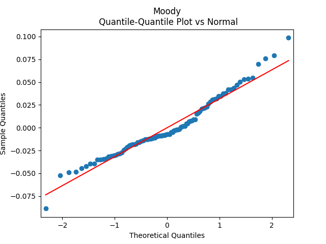
Results for innovations: They can be modeled as IID. The plots are shown below for each of the three series of residuals. First, Moody means BAA-AAA spread. Although we have strange ACF for lag 1 for absolute values, overall the plots are consistent with IID.

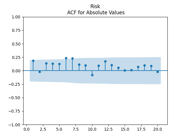
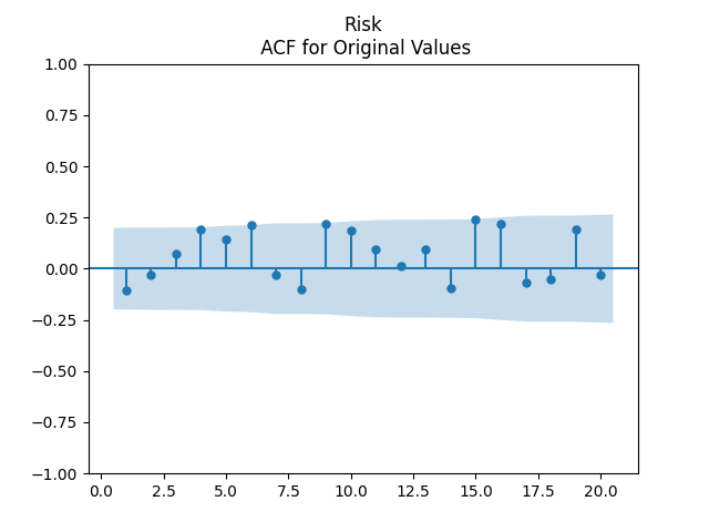
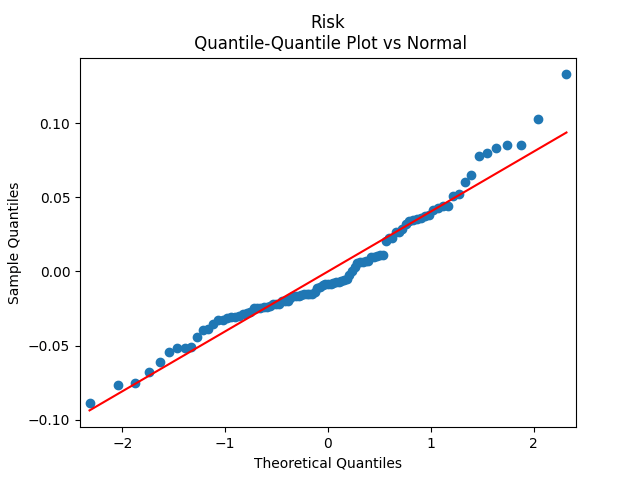
Second, Risk means AAA-Long spread. Here, we have a very good fit for IID.

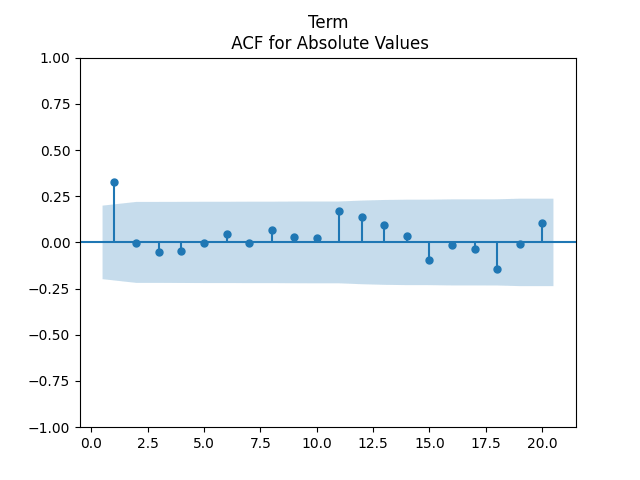
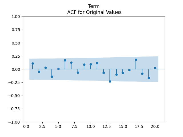
Finally, Term means Long-Short spread. We also have this strange autocorrelation at lag 1 for absolute values.

Unfortunately, we did not test the cross-correlation functions and plots, similarly to this post. We failed to do this because of lack of time, and because Python lacks a built-in function for such plots, unless you use a simple vector autoregression without volatility. But previous modeling of closely related modeling suggests that these cross-correlation functions will not be significantly different from zero.

The values of L1 norm for the first five lags of ACF from each of the 3 spreads above are:

Spread	BAA-AAA	AAA-Long	Long-Short
Original	0.445	0.539	0.328
Absolute	0.515	0.606	0.431

Recall the critical values for the L1 version of the Ljung-Box white noise test. Comparing them with our values here, we confirm we fail to reject the white noise hypothesis.

Innovations are not Gaussian, but quite close. See the quantile-quantile plots. Also, below are normality statistics.

Spread	BAA-AAA	AAA-Long	Long-Short
Skewness	0.557	0.683	-0.097
Kurtosis	0.594	0.635	1.338
Shapiro-Wilk p	1.3%	0.6%	4.3%
Jarque-Bera p	4.0%	1.0%	2.5%

PART 2: Modeling earnings growth (nominal/real) using these 3 bond spreads as regression factors, with innovations normalized by annual volatility. This model fits well, with IID but not quite Gaussian innovations.

Data: In addition to the data from PART 1, we have annual data 1927-2024: Denote December data for year t by Further, let be annual earnings 1928-2024 for S&P 90/500. These can be real (inflation-adjusted) or nominal (not inflation-adjusted). Then is log earnings growth from year to year

Model 1: We modeled it earlier as IID after dividing by volatility: But here, we model these normalized growth terms using regression versus these three spreads: Here, is a constant, is a vector, and are IID with mean zero.

Model 2: Alternatively, we can model Here we normalize residuals by volatility. Here, again are IID with mean zero, is a vector and are scalars. This is different from the first model, where we normalize growth terms but not spreads. We fit this model after dividing this equation by

Methodology: We analyze residuals for IID Gaussian, as in PART 1, using the five-point program.

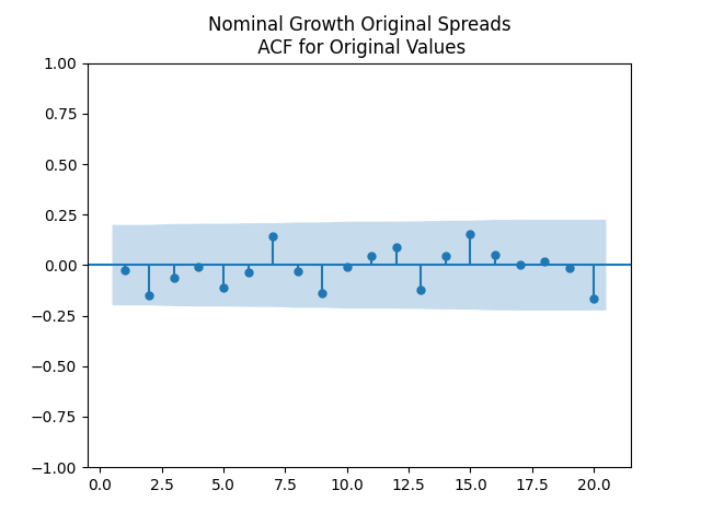
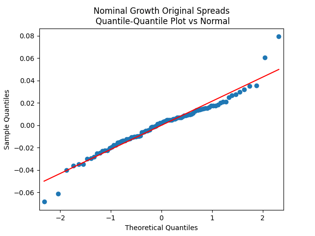
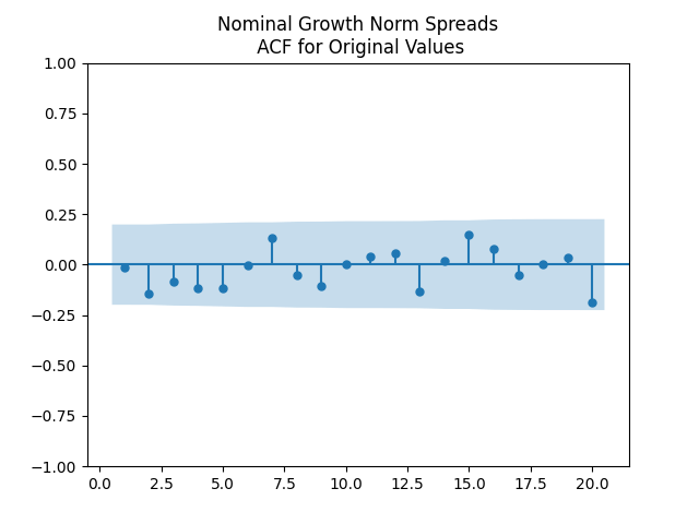
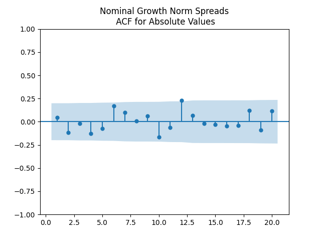
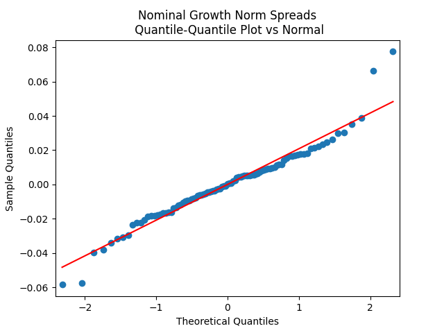
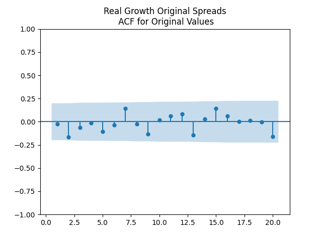
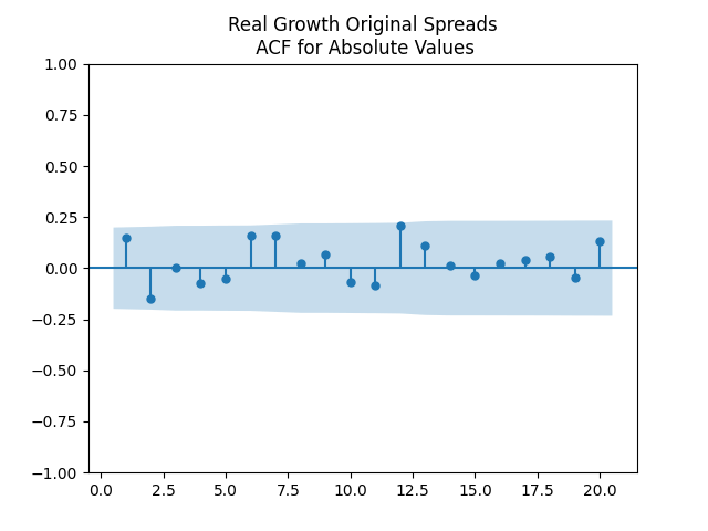
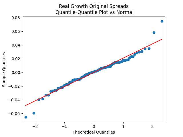
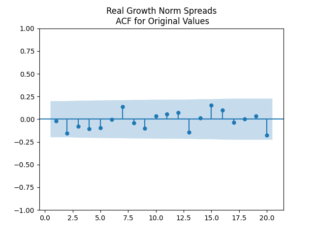
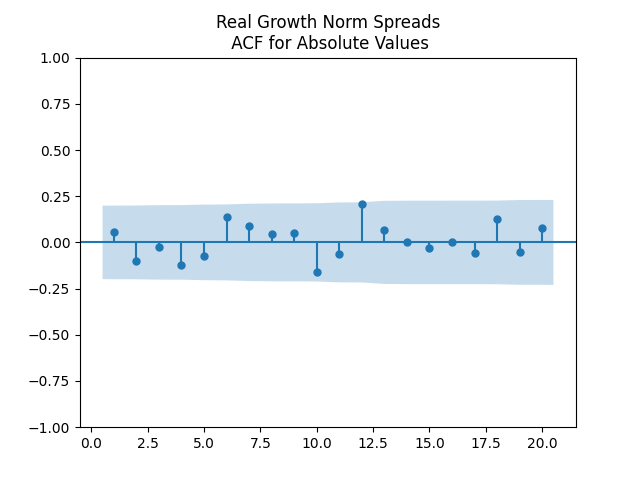
Results: All four regressions (Models 1 and 2, nominal and real) have IID residuals (judging by ACF values and plots), which are close to normal (judging by the quantile-quantile plots) but unfortunately not quite normal (judging by normality tests, skewness, and kurtosis). See plots below for Model 1 = normalized spreads, Model 2 = original spreads.

For Model 1, the only significant coefficient with is for Long-Short, judging by Student T-test. For Model 2, this is AAA-Long. All other .

For Model 1, (nominal) and (real). For Model 2, for both nominal and real.

PART 3: We model S&P annual returns (total/price, nominal/real) normalized by S&P volatility using linear regression upon three spreads: BAA-AAA, AAA-Long, Long-Short, and earnings yield. Residuals are IID Gaussian.

Data: We have 1927-2024 S&P 90/500 index data:

• end of year (last trading day close) level, 1927-2024;
• annual dividends and earnings, 1928-2024;
• annual realized volatility (standard deviation of log level daily changes), 1928-2024;
• Consumer Price Index December data, 1927-2024.

This allows us to compute four versions of index returns We allow for following options: price (excluding dividends) and total (including dividends); nominal (not adjusted for inflation) and total (adjusted for inflation). Also, we can compute earnings yield This is the ratio of annual earnings this year to end-of-year index level. See the graph below. We have a big drop in 2008 since earnings drop there much faster than index.

As above, we also have four December daily average rates: BAA, AAA, Long and Short, for 1927-2024. This allows us to compute these three spreads. We studied these spreads and used these to model earnings yield before. Denote their vector as

Model 1: Consider the linear regression Here, are IID with mean zero. Next, are scalars and

Model 2: Remove earnings yield from this regression and fit it again:

Model 3: Remove all spreads: make Then

Model 0: Remove both spreads and earnings yield: Then we get Compare with this post.

Methodology: Divide these equations by volatility and fit regressions using ordinary least squares. Use the 5-point program from Part 1 of this post to analyze residuals.

Results: Autocorrelation Function (ACF) plots for and for confirm IID. However, we still have this strange high value in lag 4, similar to the previous blog post. Computation of L1 norm for first 5 lags of ACF for and for also confirm IID.

Also, Shapiro-Wilk and Jarque-Bera tests show normality. All

Coefficients for spreads are not significantly different from zero, judging by the Student T-test, for each of four types of returns. But removing these coefficients greatly reduces We also fail to reject Judging by the value for Student T-test, these spreads are BAA-AAA, AAA-Long, Long-Short in decreasing order of importance. I think it is best to use the full version of this regression.

Conclusion: The overall model for the following quantities:

• end-of-year bond spreads BAA-AAA, AAA-Long, Long-Short:
• annual S&P 500 earnings
• end-of-year S&P 500 level
• annual realized S&P 500 volatility
• annual total S&P 500 returns

Here are independent identically distributed with mean zero, but not Gaussian.

This research is continued in the post where we consider trailing averaged annual earnings, with a window up to 10 years.