My Finance

See https://github.com/asarantsev/growth-spread for code and data.

Model explanation: Continuing research by Ian Anderson with updated data, 1927-2024, consider the following model for and which are spreads BAA-AAA and BAA-Long. Here, AAA and BAA are Moody’s December daily average rates, and Long is 10-year Treasury December daily average rates. In the previous post, we discussed that these are well-modeled as a vector autoregression of order 1, with mean reversion in the long run, if only we divide innovations and by annual volatility, computed by my other undergraduate student Angel Piotrowski. Then are independent identically distributed bivariate Gaussian.

As usual, this can unfortunately lead to ordinary least squares for regression fitting not applicable. Let us first divide each question by annual volatility, and add an intercept (constant) for completeness (because usually, linear regression includes an intercept). We get:

In the vector form, we can write this as

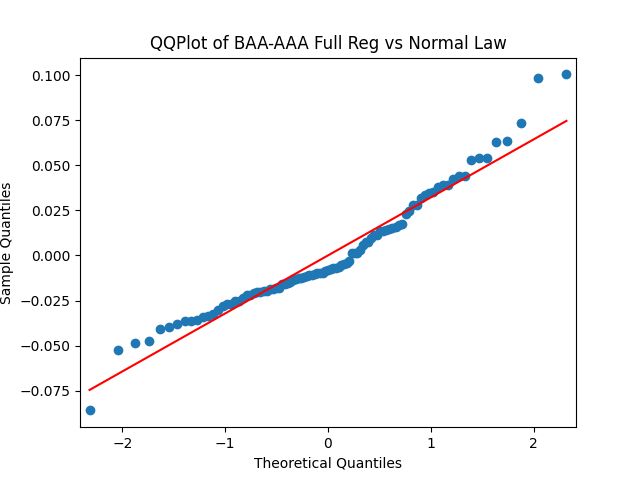
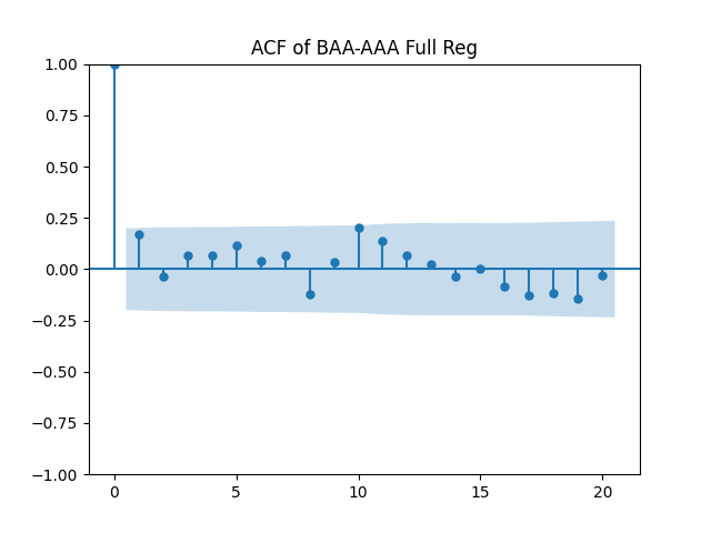
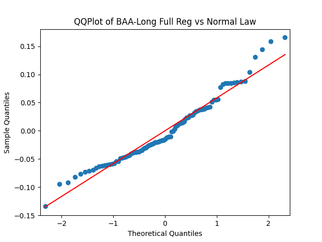
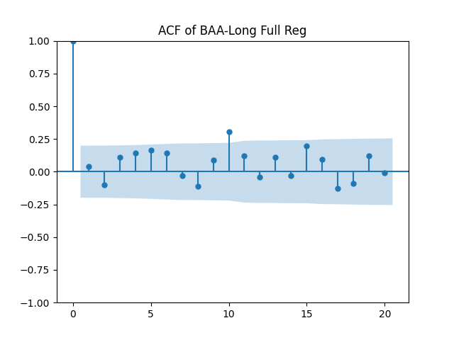
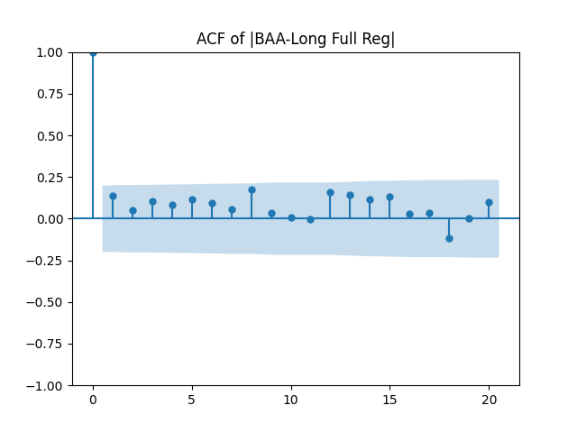
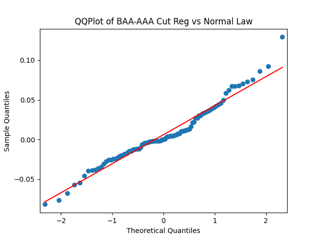
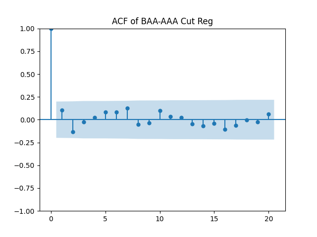
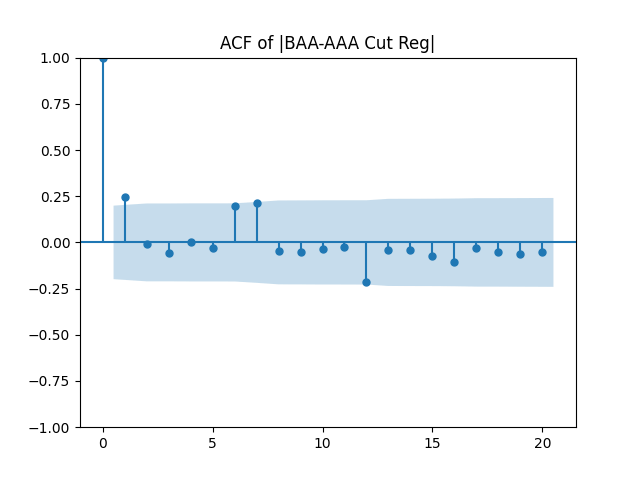
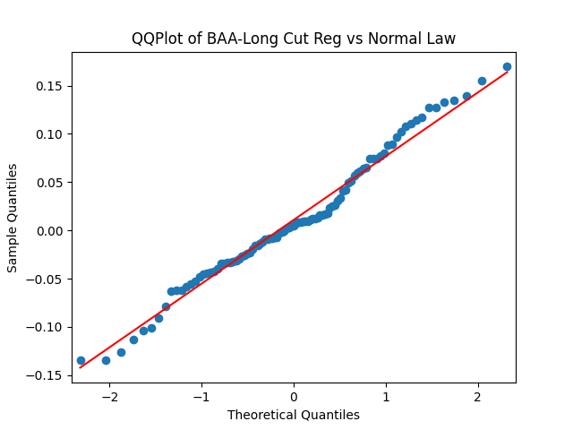
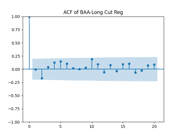
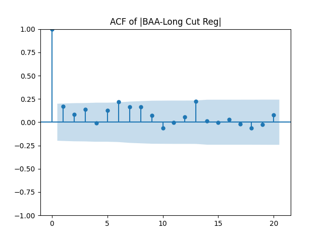
Results: Unfortunately, innovations here are further from Gaussian than in the previous post. Judging by the autocorrelation function plots for these innovations and for their absolute values: Yes, we can model as independent identically distributed. Same is shown by the L1 norms. But the quantile-quantile plots clearly say these are not Gaussian. Similarly, the Shapiro-Wilk and Jarque-Bera tests give us very low p-values.

Innovations	Skewness (Gaussian = 0)	Kurtosis (Gaussian = 0)	Shapiro-Wilk p-value	Jarque-Bera p-value	L1 norm for 5 lags ACF of original values	L1 norm for 5 lags ACF of absolute values
BAA-AAA	0.714	0.847	0.2%	0.4%	0.45	0.605
BAA-Long	0.631	0.181	1.0%	3.7%	0.554	0.487

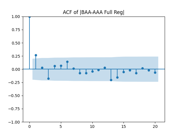
We recall that the threshold 95% value for the L1 statistic is around 63%, based on Monte Carlo simulations.

Dependence upon volatility which corresponds to the term is positive and very significant. The Student T-test gives us For both regressions,

Removing intercepts: If we do the vector model above without , we get much improved innovation sequences. Compare L1 norm values:

Innovations	Skewness (Gaussian = 0)	Kurtosis (Gaussian = 0)	Shapiro-Wilk p-value	Jarque-Bera p-value	L1 norm for 5 lags ACF of original values	L1 norm for 5 lags ACF of absolute values
BAA-AAA	0.5	0.819	2.8%	3.4%	0.375	0.342
BAA-Long	0.204	-0.203	15.9%	65.8%	0.489	0.528

The p-values for Student T-test for BAA-AAA with factor BAA-Long is 32.3% and the other way around is 43%. In principle, we could model these two spreads as separate autoregressions of order 1, but with correlated innovations.

Conclusion: For bivariate vector autoregression of order 1 applied to BAA-AAA and BAA-Long spreads, dividing innovations by volatility makes them independent identically distributed Gaussian. After that, adding this volatility as a factor in a linear regression improves the fit as judging by significant dependence, and keeps innovations independent identically distributed, but destroys their normality.