My Finance

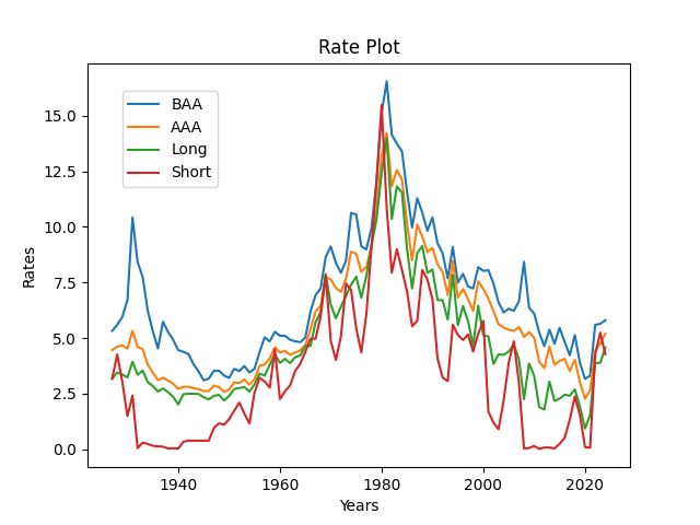
Data description: This research is an improvement of Ian Anderson’s research. See GitHub/asarantsev repository 4rates, which contains Python code, Excel data, and all generated pictures. We take four series of USA bond rates, annual end-of-year (December, monthly average) data:

• Short: 3-6 month government yields 1927-1933, 3-month 1934-now
• Long: long-term government yields 1927-1963, 10-year 1964-now
• AAA Moody’s
• BAA Moody’s

We need to take this because this is an improvement over existing Robert Shiller’s data: Hard to find long and short-term interest rates. Also, Robert Shiller’s data is average January, and our data is December. But to model next year’s stock returns, we need the data we know by the end of this year: Thus we need December, not January.

Statistical Methodology: For each series, we fit an autoregression of order 1: We analyze innovations for Gaussian IID. Next, we divide for annual volatility available for 1928-2024, and analyze for Gaussian IID.

Analysis for Gaussian IID is performed as follows:

1. Skewness (with Gaussian = 0)
2. Kurtosis (with Gaussian = 0)
3. Shapiro-Wilk normality test
4. Jarque-Bera normality test
5. Quantile-quantile plot versus the normal distribution
6. L1 norm for autocorrelation function for original values, 5 lags
7. L1 norm for autocorrelation function for absolute values, 5 lags
8. Autocorrelation function plot for original values
9. Autocorrelation function plot for absolute values

For items 1, 2, 6, 7, we use the Monte Carlo simulations giving us 95% and 99% percentiles. This allows us to make normality tests and white noise tests.

Analysis of rates: We summarize results in the table below. The sign XXXXX shows we have independent identically distributed Gaussian innovations. If we have only one of two features: Gaussian but not independent identically distributed, or vice versa, we show it. The term Success means Independent identically distributed Gaussian.

Rate	Original innovations	Normalized innovations
BAA	Independent identically distributed	XXXXX
AAA	XXXXX	XXXXX
Long	XXXXX	XXXXX
Short	XXXXX	XXXXX

Thus we can use autoregression only for BAA rates: Here the for the Student T-test. Here are independent identically distributed but not Gaussian.

Also, we apply the vector autoregression of order 1 for the vector of all four rates. Then we apply the same analysis to each of the four series of innovations. Unfortunately but not surprising, we have complete failure for all innovations. First, we present the autocorrelation and cross-correlation function plots for these four series.

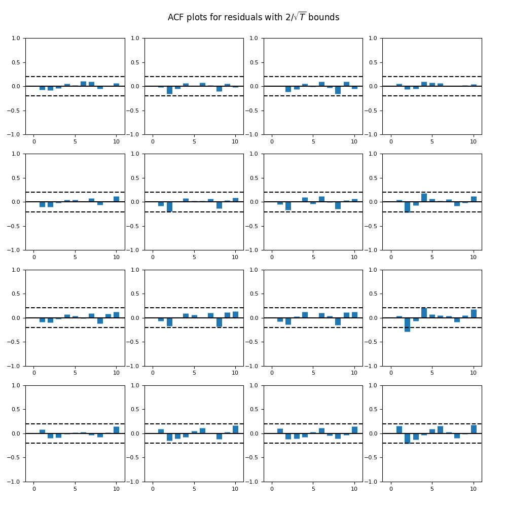
Seems like all plots correspond to white noise. But plots of absolute values of innovations show our failure. We summarize:

Rate	Original innovations	Normalized innovations
BAA	Independent identically distributed	Independent identically distributed
AAA	XXXXX	XXXXX
Long	Gaussian	XXXXX
Short	XXXXX	XXXXX

Bond spreads: Finally, we do the same analysis for spreads. There are six series of spreads.

Spread	Original innovations	Normalized innovations
BAA-AAA	Independent identically distributed	Success
AAA-Long	Independent identically distributed	Gaussian
Long-Short	Independent identically distributed	XXXXX
BAA-Long	Independent identically distributed	Success
BAA-Short	Independent identically distributed	XXXXX
AAA-Short	XXXXX	XXXXX

Let us write autoregression for BAA-AAA, AAA-Long and BAA-Long (all Student p-values are very small):

BAA-AAA: and

AAA-Long: and

BAA-Long and

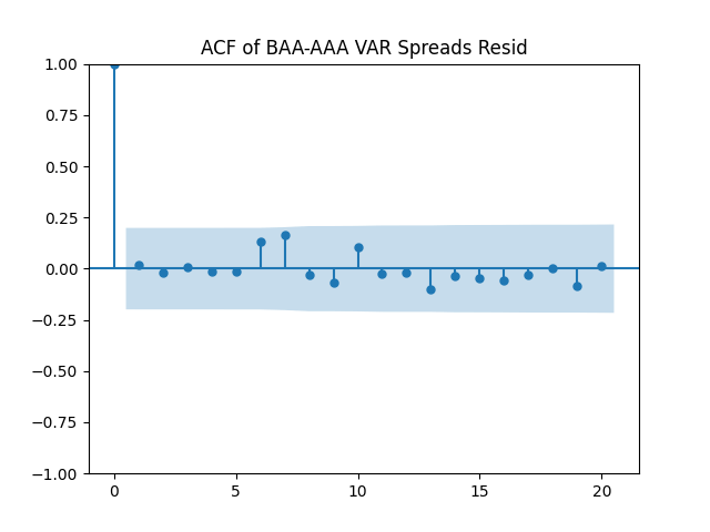
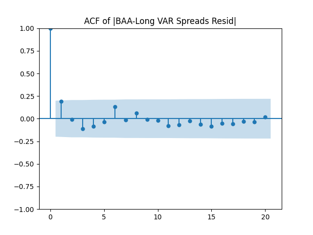
Vector autoregression for two spreads BAA-AAA, BAA-Long: We write vector autoregression for bivariate series which is BAA-AAA, BAA-Long:

Overall, it seems reasonable for us to model as independent identically distributed. See below the autocorrelation and cross-correlation plots. The correlation of its two components is 89%.

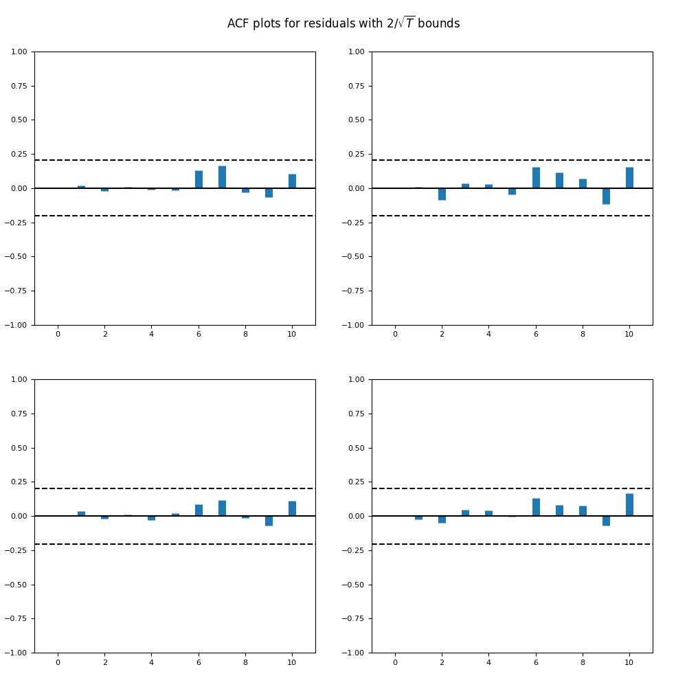
Below see plots for the first series of residuals before normalization: the quantile-quantile plot versus the normal distribution; the autocorrelation function for ; the autocorrelation function for We see it is reasonable to model as independent identically distributed but not Gaussian.

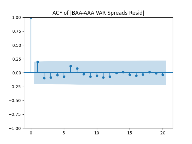
Next, we normalize these residuals by dividing them by and make the three plots for We see it is reasonable to model as independent identically distributed normal.

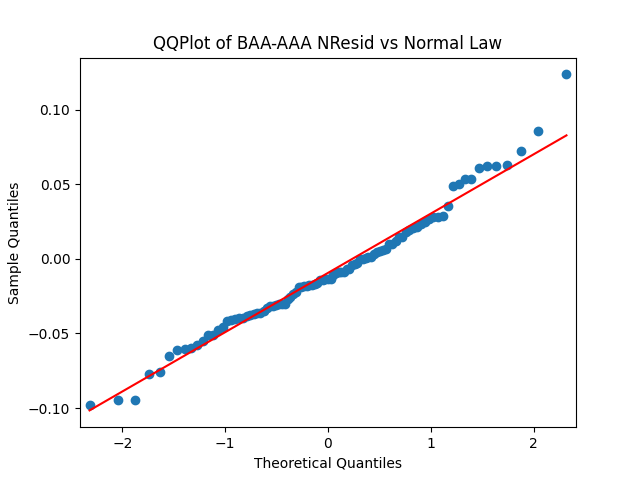
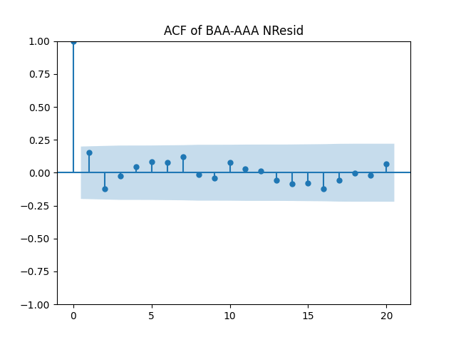
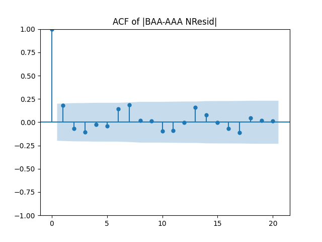
Similar results are true for . Make the three plots for this second series of residuals.

And make the same plots after division by

Conclusion. We can model [BAA-AAA, BAA-Long] as bivariate mean-reverting vector autoregression of order 1 with bivariate Gaussian innovations. All other rates and spreads do not allow autoregression modeling with Gaussian innovations.

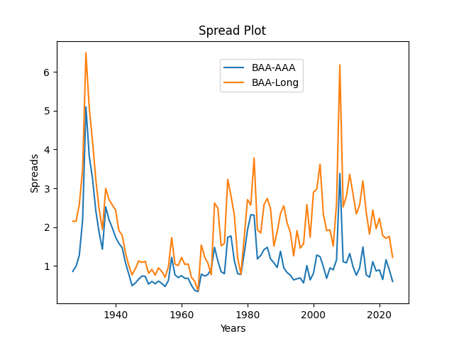
Of course, the spread between BAA rates and AAA rates is smaller than between BAA rates and long-term Treasury rates.