My Finance

In the last few days, I did a lot of research.

In the previous blog post, I have written about the simulator using only one factor: annual volatility, and two equations: for volatility and for total returns. Annual volatility was computed by my undergraduate student Angel Piotrowski as realized standard deviation of daily price returns. I multiplied it by 1000 for normalizing.

Our Model: Here, I extended it to two factors: annual volatility and annual earnings. Previously, annual earnings growth was modeled by another undergraduate student Ian Anderson. We have four equations:

• Autoregression of order 1 for logarithmic volatility
• Earnings growth divided by volatility as IID
• Price returns (excluding dividends) as linear regression with innovations = IID times volatility
• Total returns (including dividends) as linear regression with innovations = IID times volatility

These two regressions have factors: this year’s volatility and previous year’s earnings yield: last year’s earnings divided by end of last year’s index. This earnings yield is the classic valuation measure used by financial practitioners.

This model has two versions for the last three equations: nominal (not inflation-adjusted) and real (inflation-adjusted). We use four series of innovations which are multivariate Gaussian: with mean zero. Let us write these equations explicitly. Let and be earnings and volatility in year Let be the end of year index level. Let be total returns for this index, including dividends. Then we have:

Volatility:

Earnings growth:

Price returns:

Total returns:

Regression Results: Below is the table. We see that coefficients are significantly different from zero. In particular, returns and volatility have significant negative dependence. But is not significantly different from zero. Interestingly, we see that dependence of returns upon earnings yield is positive (undervalued markets grow faster) but very weak. A better measure might be cyclically adjusted price-earnings ratio, called Shiller CAPE, see future posts. This ratio is based on 10-year trailing averaged inflation-adjusted earnings.

Presumably this low prediction value is because of high volatility of earnings. For example, in 2008 earnings plummeted so much that the yield plummeted as well, thus making the markets seem overvalued. But in reality, they were undervalued, since earnings rebounded fast, and it took the markets an entire decade to rebound.

	Point Estimate	95% Confidence Interval	p-value for Student test
Real Returns	0.1655	[0.064, 0.267]	0.002
Real Returns	-0.0141	[-0.024, -0.005]	0.004
Real Returns	0.1453	[-0.903, 1.194]	0.784
Real Returns	0.1668	[0.068, 0.265]	0.001
Real Returns	-0.0136	[-0.023, -0.004]	0.004
Real Returns	0.5494	[-0.465, 1.564]	0.285
Nominal Returns	0.1693	[0.074, 0.264]	0.001
Nominal Returns	-0.0133	[-0.022, -0.004]	0.003
Nominal Returns	0.4432	[-0.537, 1.424]	0.372
Nominal Returns	0.1706	[0.079, 0.262]	0.000
Nominal Returns	-0.0127	[-0.021, -0.004]	0.004
Nominal Returns	0.8473	[-0.097, 1.792]	0.078

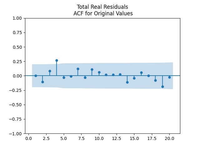
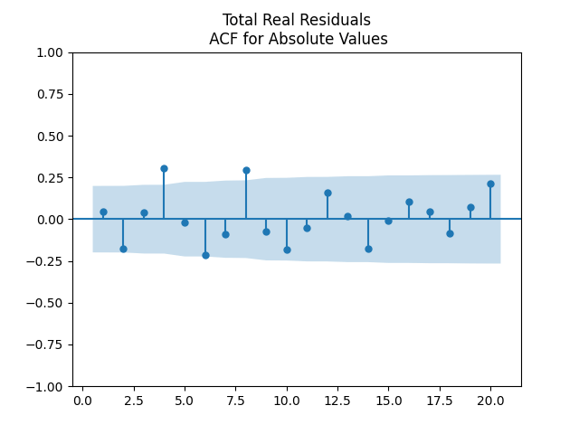
Normality: Skewness, kurtosis, and normality tests (Shapiro-Wilk and Jarque-Bera) show that residuals for price and total returns are Gaussian. However, evidence for normality of earnings growth normalized by volatility; or, equivalently, residuals The Shapiro-Wilk tests for nominal and real earnings growth give us which are 4.6% and 5.8%. The Jarque-Bera tests give us 0.2% and 0.5%. Kurtosis is especially large: 4.7 for nominal and 4.5 for real versus 3 for Gaussian.

Independence: We show below the autocorrelation functions for original values of residuals: and We pick the regression for total real returns. Evidence for IID is there but there are problems with this. We are not sure why there is large autocorrelation with lag 4. We did not apply the Ljung-Box omnibus test for the first 5 or 10 autocorrelation values. But we think it would reject the white noise hypothesis. Other regressions for other returns: price real, total nominal, price nominal, show similar autocorrelation plots for residuals and their absolute values.

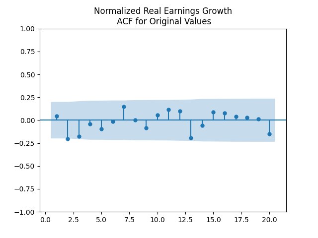
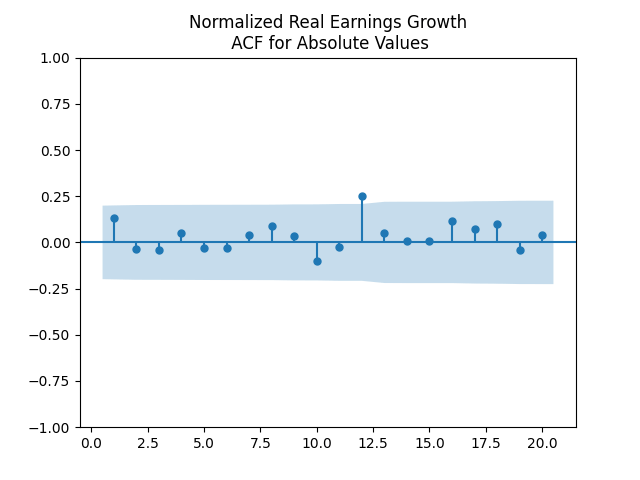
Next, the autocorrelation function plots for nominal and real growth terms show that these can indeed be modeled by IID. We show plots for real earnings growth. Nominal earnings growth have similar autocorrelation plots.

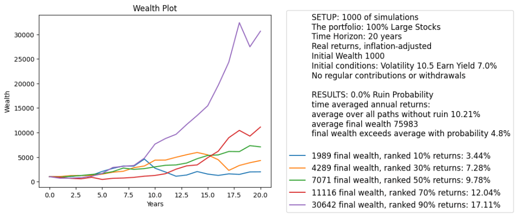
Simulation. We built a version of the financial simulator which has inputs: initial volatility, initial earnings yield, and time horizon in years. We also allow, as usual, annual contributions or withdrawals. We allow for nominal (not inflation-adjusted) or real (inflation-adjusted) versions. The code and data are available on GitHub/asarantsev repository earnings-yield-annual-simulator. We see the graph of total wealth below. This graph also shows:

• No contributions or withdrawals
• Real returns
• 20 years time horizon
• Initial volatility: 10.5 (close to historical average)
• Initial earnings yield: 7% (close to historical average)

We see that average returns over time and all simulations is 10.21%. This is much higher than historical average returns: 6.7%. This presents a problem: If we start with average data, then we should reproduce historical average returns over many simulations. We also see that with high probability returns are very large: the 90% quantile is 17.11%.

Finally, plot earnings yields for the five chosen simulations. We see that yields can become very high. In two simulations out of five, we have yields greater than 30%. Yields like this do not happen in real life.

What is the reason? We think it is because we have exponential terms in the time series equation for earnings yield Note that the log change in earnings yield can be represented as the difference between price returns and earnings growth:

Take the equations for earnings growth and price returns at the beginning of this post. Plug them into the above equation:

The change in depends on exponentially. This might lead to volatile fluctuations, especially when the yield is large. Then fluctuations are also large. This needs to be researched further.

Conclusion: We think this makes our research financially unrealistic, despite rigorous statistical analysis. A better way might be to use the CAPE or its inverse, cyclically adjusted earnings yield (using the last few years average for earnings instead of only last year). Another way might be to reproduce my research on the new valuation measure.