My Finance

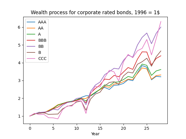
A continuation of research in github.com/asarantsev repository Annual-Bank-of-America-Rated-Bond-Data from my previous post. Consider total returns computed from total wealth process as log change: The plot of the wealth process normalized so that is given below. We see that high-yield, low-rated bonds provide more long-run returns but with much more risk.

If these were Treasury bonds and there were no risk of default, and if these were zero-coupon bonds (with only principal payment at maturity) then total returns would be equal to the rate minus maturity times rate change. See my manuscript arXiv:2411.03699. The equation is: If the bonds were having coupons, then instead of maturity there would be duration (average time of coupon and principal payments, weighted by payment size). But we add noise (innovation) terms, and an intercept:

The maturity is given in the following table, together with analysis of residuals: skewness, kurtosis, Shapiro-Wilk and Jarque-Bera normality test valued. Also, we take the sum of absolute values of the autocorrelation function for the first five lags, separately for original values of residuals and for their absolute values.

Rating		Skewness	Kurtosis	Shapiro-Wilk	Jarque-Bera	ACF of	ACF of
AAA	6.03	-2.049	5.173	0.014%	<0.001%	0.539	0.687
AA	4.89	-0.941	1.154	2.549%	5.831%	0.944	0.874
A	4.94	-0.894	1.307	7.877%	5.726%	0.977	0.704
BBB	5.17	-0.573	0.027	25%	46%	0.38	0.604
BB	3.81	-1.75	3.64	0.054%	<0.001%	0.83	0.245
B	3.12	-2.036	4.323	0.003%	<0.001%	1.17	0.653
CCC	2.55	-2.304	5.34	0.001%	<0.001%	0.9	0.716

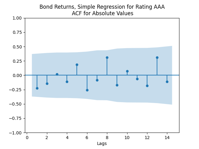
The autocorrelation function plots for and for show that these are independent identically distributed. However, the quantile-quantile plot of versus the Gaussian distribution show these are not normal, for most ratings. See the plots below.

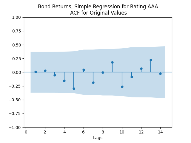
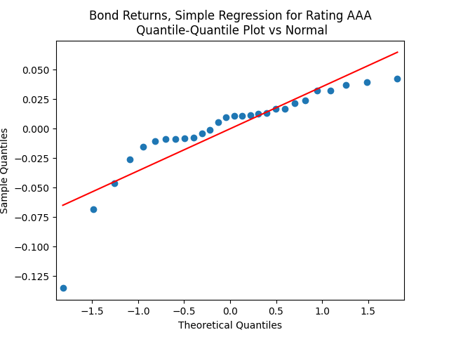
This is confirmed by the results of Shapiro-Wilk and Jarque-Bera tests, shown in the table above.

Apply the same technique as in the previous post: Normalize residuals by dividing them by annual average VIX. We get: We divide this equation by and get an ordinary least squares regression without intercept. This is not usual, so let us add an intercept:

Coefficient estimates and analysis of innovations is shown in the table below.

Rating				Skewness	Kurtosis	Shapiro-Wilk	Jarque-Bera	ACF of	ACF of
AAA	0.0661	7.0787	-0.0034	-0.737	0.576	28%	23%	0.922	0.361
AA	0.0453	5.3226	-0.0023	0.126	-0.039	46%	96%	0.57	0.761
A	0.0423	5.3423	-0.0022	-0.181	0.02	35%	93%	0.73	0.459
BBB	0.0293	5.6074	-0.0016	-0.232	-0.775	67%	62%	0.875	0.498
BB	0.0422	3.6671	-0.0024	-0.894	1.426	19%	6.3%	0.574	0.888
B	0.0682	2.9970	-0.0050	-1.562	3.479	0.397%	<0.001%	0.998	0.354
CCC	0.0712	2.6532	-0.0075	-1.588	2.649	0.072%	0.005%	0.835	0.723

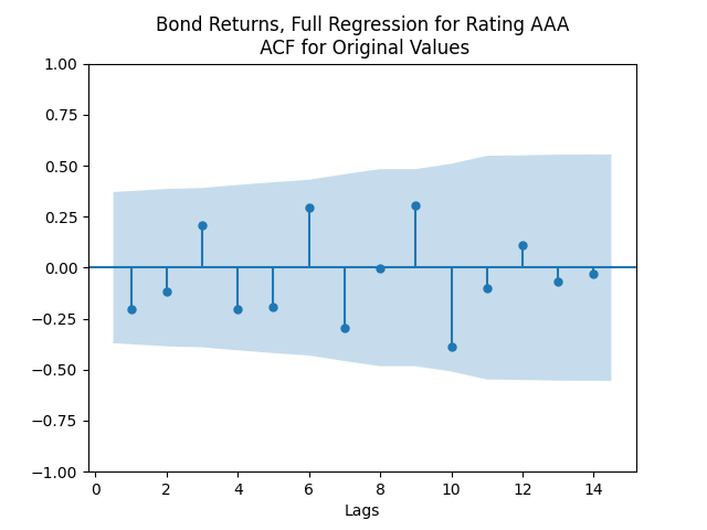
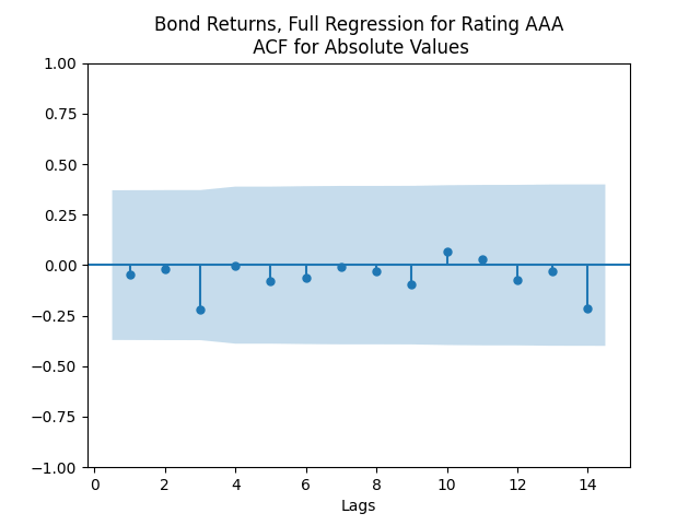
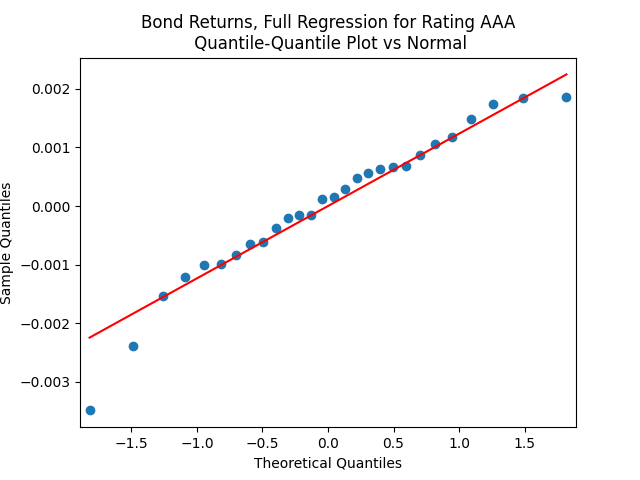
We see the residuals can be well described as Gaussian white noise for ratings BB and higher, especially well for investment-grade bonds. But for B and CCC ratings, not so much. However, judging by the ACF, new residuals (see the second table) are comparable to old residuals (see the first table) in being close to independent identically distributed. See also the following plots for AAA rated bonds:

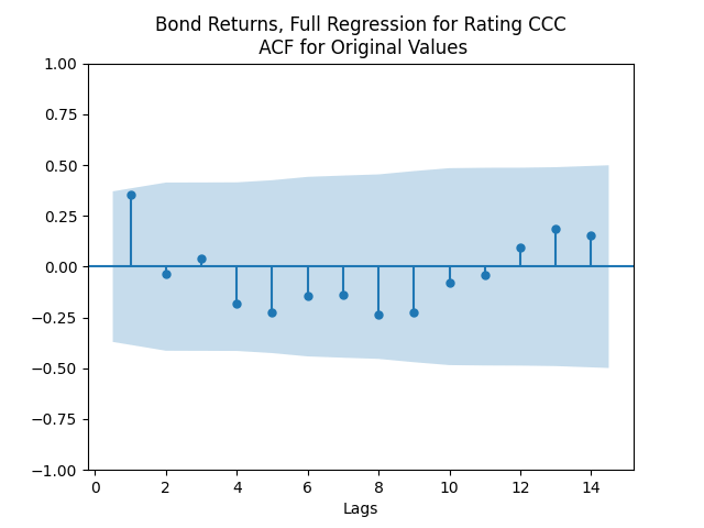
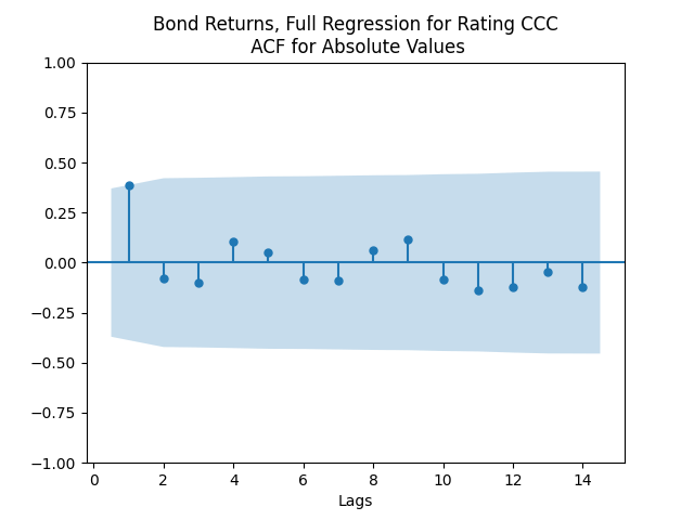
And for the lowest-rated CCC bonds the situation is different: We see that the first lag is quite significant for both version of the autocorrelation function.

Combining the model above with the results of the previous post, we get the trivariate model:

And the wealth process is given by It is possible to show this model for is long-term stable and ergodic, because for each of seven ratings, We have done this for in our previous work. For this is trivial.

Next, for ratings BB and above, the trivariate innovations sequence is modeled as independent identically distributed trivariate Gaussian. Our code find the covariance matrix for these. We do not put it here but an interested reader can run the code.