New Bubble Measure Work Replicated

This is the work with my undergraduate student Angel Piotrowski. She used her annual volatility data 1928-2023 to replicate my previous work published on arXiv and discussed in my previous blog entry about the new valuation measure for the Standard & Poor 500 and its predecessors. She used the end-of-year S&P 500 close trading price instead of the January S&P 500 daily close averaged price used by me. She used December Consumer Price Index (CPI) data instead of me using January CPI. And she used data only 1928-2023 instead of my work 1871-2023. But this almost a century of data is still enough to make conclusions.

First, adjust earnings for inflation and consider the trailing average  E(t) of earnings for the last 5 years. This is similar to the classic Campbell-Shiller approach, when the cyclically adjusted price-earnings ratio (CAPE) features last 10 years of earnings. But we chose 5 years to make room for more data. Next, take inflation-adjusted wealth  S(t) at end of year  t. Consider the linear regression

 \ln S(t) - \ln E(t) - ct = a + b(\ln S(t-1) - \ln E(t-1) - c(t-1)) + \delta(t).

This has the meaning of subtracting the trend from relative growth of wealth over earnings. Historical earnings averaged 1-2% per year and wealth growth is around 6-7% per year so the value for the trend  c must be 4-5%. This equation shows that after detrending, this is the classic autoregression of order 1. We can rewrite this in the more standard ordinary least squares regression form:

 Q(t) = a + bc + t(c - bc) + (b-1)(\ln S(t-1) - \ln E(t-1)) + \delta(t),

where we define for short notation the quantity which we called implied dividend yield:

 Q(t) := \ln S(t) - \ln E(t) - \ln S(t-1) - \ln E(t-1)

This gives us  a + bc = 0.1351 and  c - bc = 0.0101 and  b - 1 = -0.1307. All three coefficients are significantly different from zero: Student T-test gives p values  0.1\%, 2.9\%, 1.9\%. But the Jarque-Bera test shows that innovations are not Gaussian:  p = 0.1\%. This is confirmed by the following quantile-quantile plot below. But the autocorrelation function plots for  \delta(t) and for  |\delta(t)| below show that these are independent identically distributed.

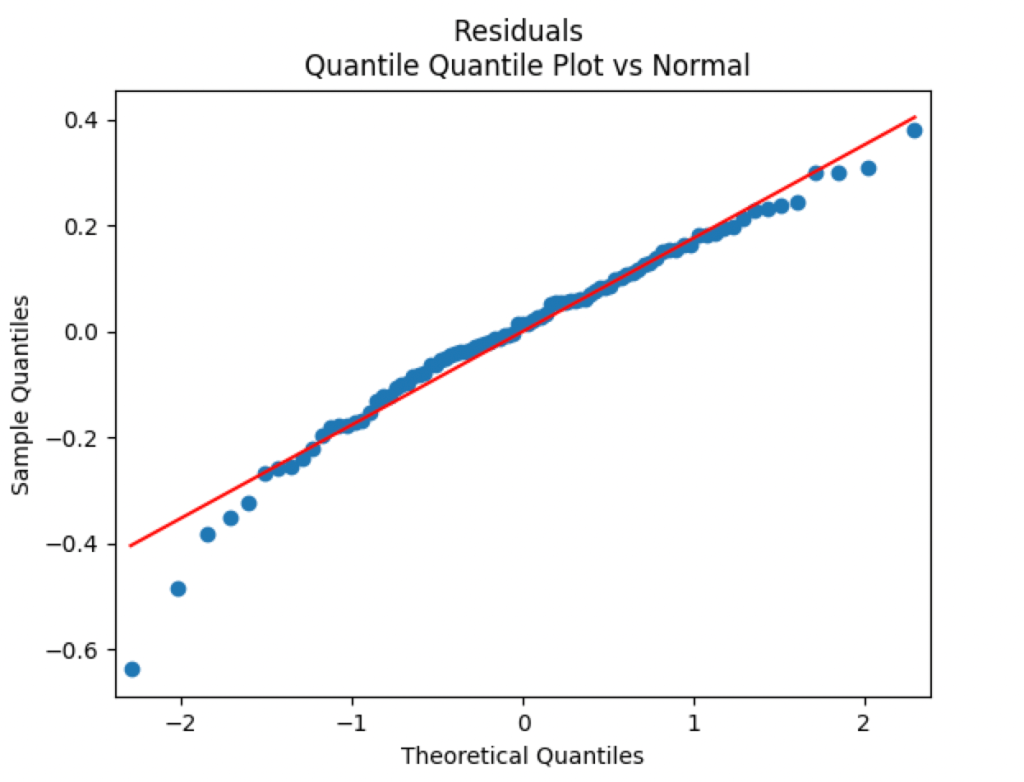
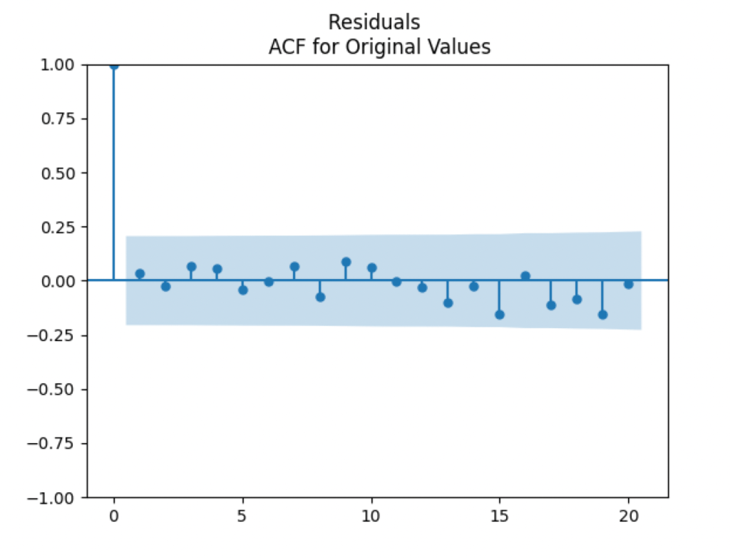
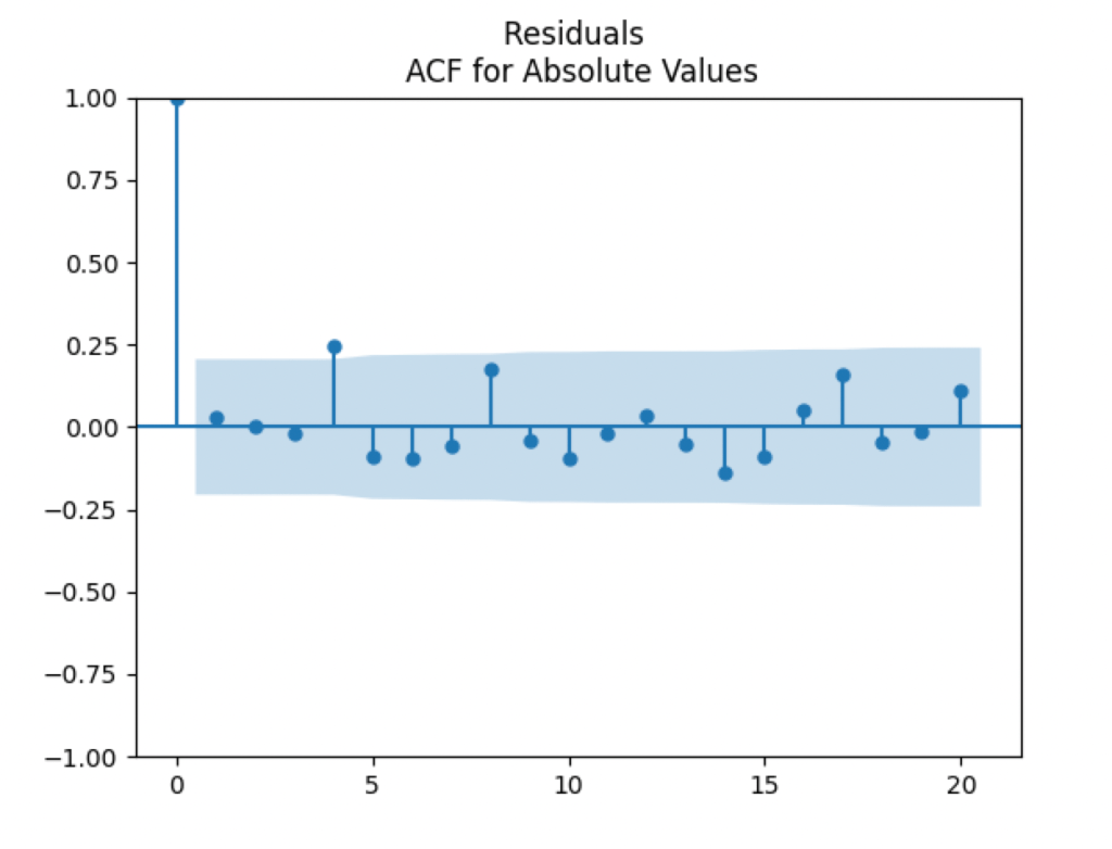
This stays in contrast with our original research, when residuals (innovations) are independent identically distributed and Gaussian. Further research will include extending this to years 2024 and 1924-1928 when we have total returns and volatility data for shifted years.

The GitHub repository New Valuation Measure Replication contains code, data, and these graphs.

Published by


Responses

  1. My bubble measure work – My Finance

    […] with annual volatility which she computed previously. Here I try to explain my research. In a further post, I will explain Angel’s […]

    Like

  2. New Valuation Measure Replicated + Volatility – My Finance

    […] continue the previous post of joint work with my undergraduate student Angel Piotrowski. Consider my work arXiv:1905.04603. We […]

    Like

  3. Annual simulator with volatility and the new valuation measure of S&P 500 – My Finance

    […] GitHub repository, I made a simulator of the Standard & Poor 500 annual total returns using the new valuation measure and annual volatility with inputs: Nominal or Real, and averaging window ranging from 1 to 10 […]

    Like

  4. Simulators – My Finance

    […] the model with this new valuation measure and the three spreads, and create a simulator for […]

    Like

Leave a reply to My bubble measure work – My Finance Cancel reply