Make S&P Returns IID Gaussian

My undergraduate student Angel Piotrowski continued her work, started with annual volatility 1928-2023. First, she updated the annual realized volatility for 2024. The resulting series 1928-2024 is still well modeled by log Heston model, see another post. The research in this post is done in GitHub/asarantsev repository.

Then she computed annual returns of S&P 500 (and its predecessor, S&P 90) 1928-2024 in four versions:

  1. nominal (not adjusted for inflation) or real (adjusted for inflation);
  2. price (due only to price changes) or total (including dividends paid).

We take nominal annual dividend:  D(t) and December Consumer Price Index  C(t) We take the price  S(t) at the close of the last trading day of the year  t. Price returns are computed as  \ln\frac{S(t)}{S(t-1)} and total returns are  \ln\frac{S(t) + D(t)}{S(t-1)} for nominal versions. But for real versions, we need to subtract  \ln\frac{C(t)}{C(t-1)} from each of these. You see that all returns are logarithmic (geometric), so there is no problem of compound interest. If wealth at end of year  t is  \mathcal W(t) then  \mathcal W(t) = \exp(Q(1) + \ldots + Q(t))\mathcal W(0) where  Q(t) is returns during year  t.

In each of these four cases, returns are IID but not normal. However, dividing them by volatility keeps them IID but makes them normal. Just to illustrate, let us take real price returns  Q(t)

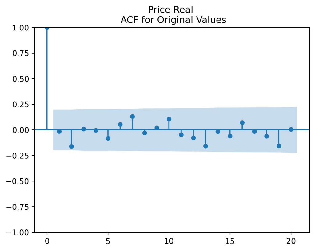
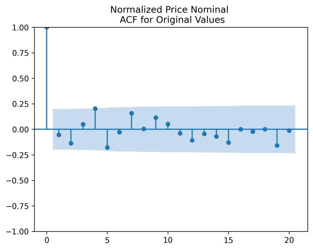
The autocorrelation function for  Q(t) (left panel) and for  |Q(t)| (right panel) show these are close to zero. So it is reasonable to model these as independent identically distributed random variables. However, the below quantile-quantile plot versus the normal distribution shows these are not normal.

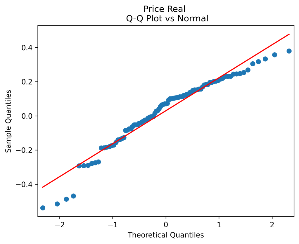
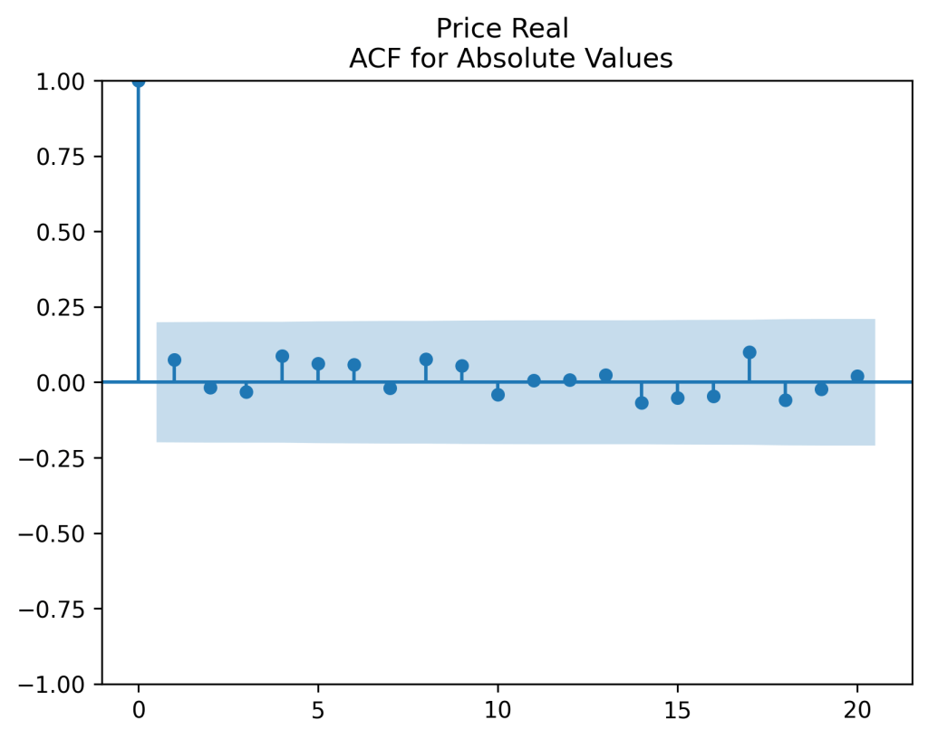
Next, repeat this analysis for normalized

And see that  Q(t)/V(t) are also well modeled as independent identically distributed. But unlike the previous example, the quantile-quantile plot shows that  Q(t)/V(t) is Gaussian:

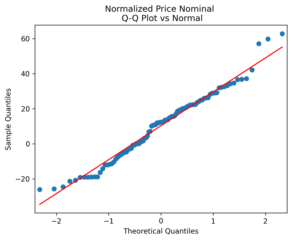
This is confirmed by results of two statistical tests for normality: Shapiro-Wilk and Jarque-Bera. See their p-values below. One can clearly see we reject normality hypothesis for original but not normalized returns, for all four versions of returns, and for each of two tests.

ReturnsOriginal Total RealNormd
Total Real
Original Total NominalNormd Total NominalOriginal Price RealNormd Price RealOriginal Price NominalNormd Price Nominal
Shapiro-Wilk p0.0016420%0.0002711%0.0008728%0.0000911%
Jarque-Bera p0.0062763%0.0000560%0.0021786%0.0000060%

Published by


Responses

  1. Financial Simulator, Current Version – My Finance

    […] from with mean zero and known covariance matrix. This follows the old blog post, and is similar to Angel Piotrowski’s research. See also large vs small […]

    Like

  2. Financial Simulator, Annual Version – My Finance

    […] we discussed its currently published monthly version. This is a simplified version based on work by Angel Piotrowski. Here we do not have any bond rates or spreads, any earnings or dividends. We have only annual […]

    Like

  3. Earnings Yield, 3 Bond Spreads, Annual Returns – My Finance

    […] Make S&P Returns IID Gaussian […]

    Like

  4. To Do List – My Finance

    […] repository Inflation-Modeling-1928-2024 for data and code. Strange, because we have both nominal and real returns divided by volatility modeled as IID Gaussian. So the difference between them: inflation/volatility should be IID […]

    Like

  5. Stock Returns vs BAA – My Finance

    […] research of the four bond rates, we model normalized total returns of S&P (nominal or real) as a regression upon the BAA rates at the end of last year, and the change in BAA […]

    Like

  6. Updated Simulator for Rate and Volatility – My Finance

    […] normalize the two stock returns by dividing them by annual volatility. But we do not normalize the bond returns. We have the following equations for […]

    Like

Leave a comment