My undergraduate student Angel Piotrowski computed annual volatility for Standard & Poor 500 (and its predecessor, Standard & Poor 90). For each year 1928 — 2023, she took daily index values with day in this year, and computed log returns Then she computed standard deviation of these log returns for day in any given year. Let be this standard deviation, usually called volatility, for year The data is available on my web page.
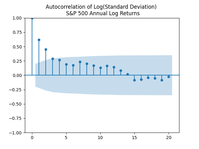
Next, Angel created a time series model for this volatility: Autoregression of order 1 on the log scale. The motivation comes from plotting the autocorrelation function for It is defined as This looks like an autocorrelation function for an autoregression of order 1.
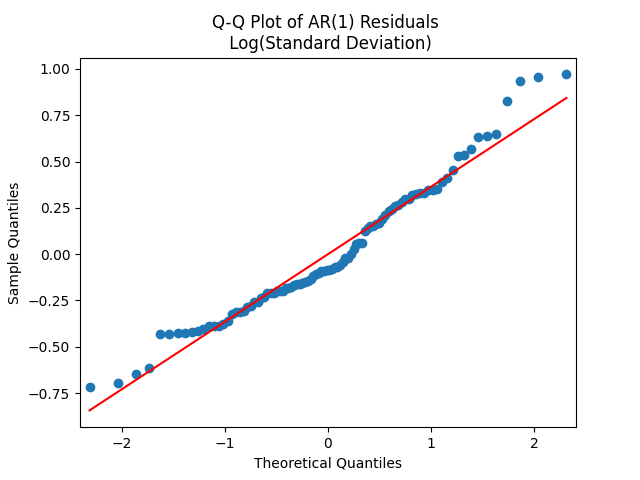
Here is the equation for this autoregression: with and Let us test whether the innovations are Gaussian. Apply the quantile-quantile plot versus the normal distribution. This looks like pretty close to a Gaussian law!
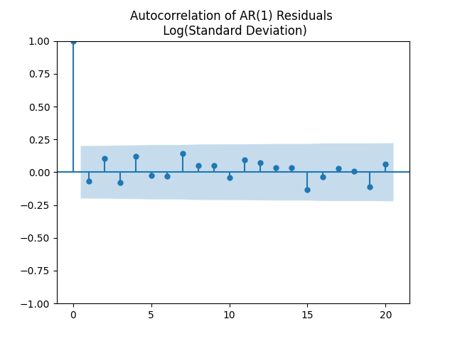
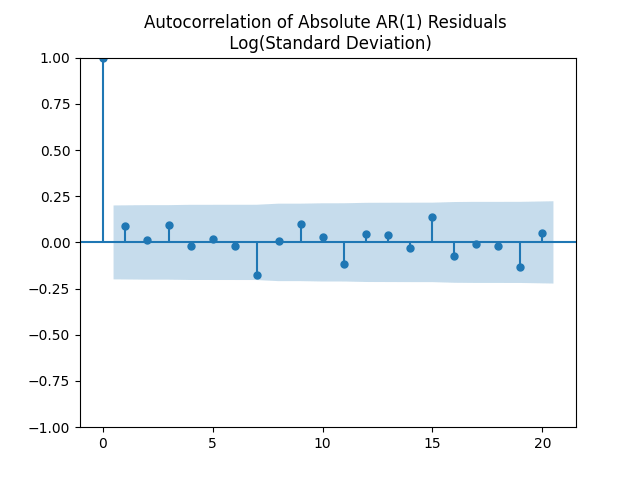
Next, plot the autocorrelation function for innovations and another plot of an autocorrelation function for their absolute values to see that they correspond to white noise.
Thus the model fits well: We have numerical estimates Therefore, this autoregression has a stationary distribution, or an invariant probability measure, such that Angel has computed that mean and variance of this stationary distribution.
Dividing by volatility improves bond spread models – My Finance
[…] This work is of my undergraduate student Ian Anderson using the annual January data for American bond rate spreads. It uses annual volatility data complied by my other undergraduate student Angel Piotrowski. See the previous post. […]
Annual Earnings and Volatility for Standard & Poor 500 – My Finance
[…] This work was done by my undergraduate student Ian Anderson, using the volatility data computed by my other undergraduate student Angel Piotrowski, see the previous post. […]
Annual dividend growth terms does not become white noise after dividing by annual volatility – My Finance
[…] or real) are not Gaussian white noise. But after dividing these growth terms by annual volatility (computed by my other undergraduate student Angel Piotrowski) they indeed become Gaussian white […]
[…] undergraduate student Angel Piotrowski continued her work, started with annual volatility 1928-2023. First, she updated the annual realized volatility for 2024. The resulting series 1928-2024 is […]
[…] undergraduate student Angel Piotrowski updated annual realized volatility for 2024. Previously she computed it for 1928-2023, each year. She took log change in daily closing prices of the Standard & Poor 500, or its predecessor, […]
New Bubble Measure Replicated with Stochastic Volatility – My Finance
[…] is the work by my undergraduate student Angel Piotrowski. She used her annual volatility data 1928-2023 to replicate my previous work published on arXiv and discussed in my previous blog entry about the […]
S&P 500 Returns using Earnings Yield & Volatility – My Finance
[…] using only one factor: annual volatility, and two equations: for volatility and for total returns. Annual volatility was computed by my undergraduate student Angel […]
S&P 500 Annual Returns with CAPE and Volatility – My Finance
[…] much better than the annual price-earnings ratio, or equivalently, annual earnings yield. We added annual volatility to the classic Campbell and Shiller’s research and much improved it. Now we have a dynamic […]
Annual simulator with volatility and the new valuation measure of S&P 500 – My Finance
[…] a simulator of the Standard & Poor 500 annual total returns using the new valuation measure and annual volatility with inputs: Nominal or Real, and averaging window ranging from 1 to 10 years. We can input time […]
[…] This is higher than the long-term average 10.51, or the 2024 volatility, which is 7.98. See the original post with computations of Angel Piotrowski for 1928-2023 and its previous update for […]


Leave a reply to Annual Earnings and Volatility for Standard & Poor 500 – My Finance Cancel reply