My Finance

A financial econometrician often hopes against hope that returns exhibit the following properties: (A) normal, following the bell curve; (B) IID, meaning independent identically distributed. Unfortunately, this is almost never true.

Here, let me describe a nifty trick: Dividing each data point by the standard deviation normalizes the data. The standard deviation of stock market returns (in financial econometrics this is called volatility) is not constant over time. Periods of economic calm and steady growth when volatility is small alternate with economic crises and financial crashes when volatility is large. It is not clear that dividing by overall volatility makes sense.

Another way to say is that volatility is stochastic: It is a random process by itself. How to extract this stochastic volatility, and how to model it? Here autoregressive conditional heteroscedastic (ARCH/GARCH) models are very useful. They model dependence of current volatility upon the past volatility and returns, with fixed number of lags. These are widely used in Quantitative Finance, often combined with classic linear autoregressive and moving average (ARMA) models. Every time series of returns would have

By chance, we discovered another trick, which obviates the need for GARCH-type models and allows to simply reduce all it to a couple of linear regressions. The miracle is that we can observe volatility independently and separately from the main time series!

Enter VIX, the index created and maintained by the Chicago Board of Options Exchange. Options are contracts which give the holder the right (but not the obligation) to buy or sell a stock or a stock index in the future (at a maturity) at a predetermined price (the strike). The celebrated Black-Scholes formula computes the option price based on current stock price, the strike price, the maturity, and the volatility.

Lost of options are traded in Chicago based on S&P 500. Comparing the market price of each option at a given moment, we solve the Black-Scholes formula backward and find the unknown volatility. This is called the implied volatility. Taking a weighted average of all options, we get the overall implied volatility of the index, which is called VIX. It was computed daily for S&P 500 from the start of 1990, and for S&P 100 (a subset of S&P 500) from 1986.

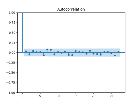
Below is the ACF plot. Take monthly returns of Wilshire Total Stock Market Index, including dividends, from 1990. Below is the plot of their autocorrelation (correlation between month and month , for each ) All correlations are very small and lie within a narrow blue band. This blue band is the fail-to-reject region, where you do not reject the null hypothesis that all returns are IID. It looks like this is, in fact, IID.

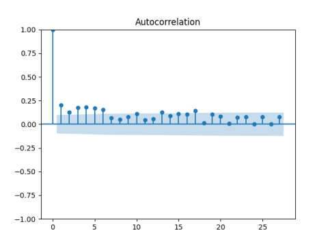
However, if we take autocorrelations for the absolute values, this is not IID anymore!

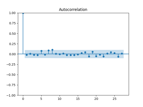
Finally, if we divide total returns by monthly average VIX, we get the autocorrelation functions for returns to be well-behaved, that is, corresponding to IID.

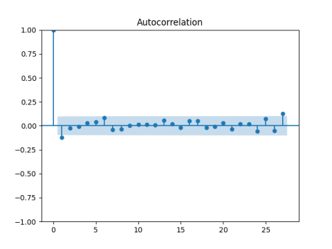
And for their absolute values as well.

We can have without autocorrelation: , but with autocorrelation. In this case, plotting autocorrelation for will give us a false impression that is IID. This would be true if were Gaussian, because for these uncorrelated means independent. Unfortunately, many times data in finance is NOT Gaussian, they have heavy tails!

We discussed in the last post the model , where IID and is auto regression or another mean-reverting process, independent of . Then X have zero autocorrelation, but have positive autocorrelation. Indeed, for crisis times V(t) is large and then is large, and thus and are both large.

When analyzing financial and economic data, one should always be mindful of this possibility. If we checked autocorrelation for both and , and both are zero, then it makes sense to assume X are IID.

We can also apply white noise tests to and to separately.

Consider correlations of ; correlation of ; etc. correlation between . Are they all close to zero? We can test them separately, or combine them (sum of absolute values, sum of squares, or another function = statistics). This gives us Box-Pierce, Ljung-Box, and any other white noise test.

Doing the same for instead of , we can reject or fail to reject white noise for .

I created combined test (omnibus or portmanteau) to test and simultaneously. See the article IID Time Series Testing (2023) in Theory of Stochastic Processes, published by the Ukrainian National Academy of Sciences.

 Moreover, it makes them normal, or much closer to normal than originally! This is true by statistical tests of normality (Shapiro-Wilk, Jarque-Bera, or others) and by the quantile-quantile plot (QQ) vs the normal law.

Finally, these properties work for any well-diversified factor market portfolio: Small, Value, Large Growth, and so on. VIX was created from S&P 500 options, but it works for indices, portfolios, and funds other than S&P 500.

Of course, the mean, variance, and other statistics of normalized returns will be different for two different portfolios. But normality and independence stay.

Portfolios are many, but volatility is universal!