Features: This is NOT a stationary model. All innovations are IID Gaussian, tested by Shapiro-Wilk and Jarque-Bera normality tests, and by the Ljung-Box test for 5 and 10 lags for original and absolute values of innovations.
Updates:
Volatility and S&P returns data thanks to Angel Piotrowski and Ian Anderson, 1928-2025
Rate data for BAA and 10-year Treasury extended back to 1925 from 1927
New versions of the main model: For international stocks, its own dividend-based valuation measure rather than rely on US-based; for Treasury bonds, use actual returns data from SBBI or FRED to compare with predicted returns from Damodaran’s formula
Smaila Amoanu helpfully scanned annual (total, nominal) long-term government and corporate bond returns 1926-2015.
I augmented the corporate bond returns by adding 1976-2025 Novel Investor data. The previous model still holds, although without volatility! with unfortunately very low .
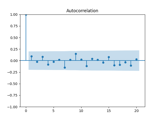
But are Gaussian IID, judging by the Ljung-Box test for 5 and 10 lags for and and by the Shapiro-Wilk and Jarque-Bera tests. The code is available here.
Also, we can analyze long-term government returns. The regression of 1926-2015 similar to the above produces duration slightly less than 9 and but with residuals which are NOT Gaussian IID. Division by volatility does not improve the fit. See the GitHub repository. But we simply switch to deterministic generation of returns of Treasuries but with 10-year maturities. Or maybe with 9-year, since we had duration around 9 in the above regression?
Also, in the new data file in the new repository https://github.com/asarantsev/Bayes9 we extended BAA and Long rates data from 1927 to 1925, two additional years. And we rewrote regressions to fit it.
Introduction. We combine the old analysis of four bond rates and six spreads (with extended and updated data, using autoregression and annual volatility, abbreviated later as VAP) with our new tool, the Yeo-Johnson transform (abbreviated later as YJX). We wish to answer whether switch to IID Gaussian innovations can be done using YJX not VAP.
Data. We take augmented December annual average rate data, all available in Github repository. All data is taken from the usual website, Federal Reserve Economic Data. These are:
Short-term Treasury rates, 1920-now
Long-term Treasury rates, 1925-now (from 1960 this corresponds to 10-year Treasury rates)
Moody’s AAA and BAA corporate bond rates, 1919-now
Analysis. We take data which is either rate or spread, with or without logarithms.
We run autoregression
We test and using Ljung-Box tests for 5 or 10 lags, and we accept IID only if all four tests give us value greater than 5%.
We apply the Shapiro-Wilk and Jarque-Bera tests for and we accept Gaussianity only when both tests give us value greater than 5%.
We divide and apply Steps 2-3 again.
We apply the Yeo-Johnson transform to and fit the autoregression
We test much like we tested in Steps 2-3.
We divide and apply Steps 2-3 again.
Results: Unfortunately, success in making these IID Gaussian is achieved using YJX only for spreads BAA-AAA, BAA-Long and some combinations of logarithms. But not for the rates themselves. Thus we cannot model bond markets without VAP.
But we are interested only in the time series modeling of volatility, since the normalized monthly returns are already IID Gaussian. Thus we apply the autoregression of order 1 to the transformed log VIX and analyze innovations of this autoregression.
Results: Shapiro-Wilk and Jarque-Bera for transformed log volatility, with However, autoregression innovations are IID but not Gaussian, both normality tests give extremely low values.
Here we describe the final steps we make to complete the simulator, first as a collection of Python files, later an online web app.
Make available classic (frequentist, with fixed point estimates for the covariance matrix of regression residuals and for regression coefficients) and Bayesian (what we called Bayesian-lite, with fixed point estimates for the covariance matrix of regression residuals but objective Bayes inference for only regression coefficients) options.
Make two versions of the model for stocks: simple (with only volatility as factor for international developed and emerging stocks, but also BAA corporate bond duration and the new valuation measure based on dividends for domestic stocks) and complete (with BAA corporate bond duration for all three stock asset classes, and the new valuation measure for both domestic and developed, but not emerging stock markets).
Make two versions of the model for bonds: simple (with Treasury long-term bond returns modeled as a deterministic function of this and last end-of-year rates) and complete (with noise components there, based on historical returns of 7-year zero-coupon Treasury bonds from 1962).
All eight versions of the model must have 10000 simulations. Moreover, all coefficients and covariance matrices, including objective Bayes inference, encoded directly in the Python code, not inferred via reading external data file or separate fitting of regressions. The latter takes some time, and while this does not seem to be so much, it does take extra 3-4 seconds on my local computer, which translates into 1-1.5 seconds on the web app (which is generally 3 times faster than my local computer). The difference between say 1.5 and 3 seconds is huge for the casual user.
There must be a separate Python file main.py which combines simulations from each of 8 chosen models and giving this graphical output, as well as a document about the exact equations and verification governing the chosen model.
A separate file bayesOLS.py contains objective Bayes simulation of regression parameters and simulation of noise terms, where we assume the standard error is constant. Finally, the inverse transform is coded in YJX.py.
We were very positively surprised that it takes such a short time. Only 10 seconds on my office computer. But the previous version without reading and fitting the data takes only 2 seconds on my office computer. Maybe we can multiply time by 5?
Update: I found a mistake, since I forgot to add correlation between the two innovation series. We need to: (a) simulate the two innovation series as bivariate Gaussian with mean zero vector and the covariance matrix which matches the empirical covariance matrix; (b) use one-dimensional innovations as an argument in the regression simulation functions.
Update: I used a more rigorous method of runtime count on my personal notebook. Then the old and new simulators generally take 6.5-7.0 seconds to run, both with 100 and 10000 Monte Carlo simulations. But this is strange that reading the data, fitting regressions etc and running these multiple Gaussian random variables seems not to make a difference! Why?
Update: I ran it on my office computer, both take around the same time. I think about 2 seconds. Crazy!
Conclusion: For us this is very good news since we now can proceed with the new simulator.
0. First Remarks. We need to use the Yeo-Johnson transform, not the Box-Cox transform to make data normal, since we need to ensure data can be both positive and negative. When we run modified random walk and autoregression simulations, we can always get outside of set bounds where the inverse Box-Cox transform is defined. We succeeded in this. And we can run simulations of such transformed volatility, and transform it back using the inverse Yeo-Johnson transform, no problem.
First, we must transform log volatility, then fit the autoregression. We should not first fit the autoregression for log volatility, then transform the residuals. This would give us IID Gaussian data, but will not allow us to make objective Bayes inference for linear regression. Transforming the original data first allows us to simulate regression coefficients and standard errors.
The code and data are given in this new GitHub repository.
1. Simulation Description. We fit a one-factor model for stock returns (nominal, total, geometric) for three asset classes:
US stocks (domestic, measured by S&P 500)
International developed markets (measured by 88% MSCI EAFE + 12% MSCI Canada)
International emerging markets (measured by MSCI EM)
Of course, for the latter two, we have less data: 1927-2025 for US stocks, 1970-2025 for developed, and 1988-2025 for emerging. Therefore, we expect Bayesian inference to make a difference. For each of 3 classes, we have two choices:
Keep volatility original, as is
Apply the Yeo-Johnson transform
We apply three modes of statistical inference, following this blog post:
Classic (frequentist, with point estimates for the covariance matrix of innovations and regression coefficients)
Bayesian lite (fixed covariance matrix for innovations, objective Bayes posterior for regression coefficients)
Bayesian full (fixed correlation matrix for innovations, objective Bayes posterior for standard errors and regression coefficients)
For each of the 18 experiments, we run 10000 Monte Carlo simulations for 20 years. We return 10 results:
For average returns over 20 years, mean, stdev, and percentiles 10, 30, 50 (=median), 70, and 90.
For 3%, 4%, 5% withdrawal rules with 4% annual arithmetic increase to adjust for inflation, the ruin probability.
2. Conclusion. We do not see much difference in ruin probability. But a lot of difference in lower quantiles and in the median. However, not much difference between Bayesian-lite and Bayesian-full. Therefore, later we simply consider Bayesian-lite mode as an alternative to the frequentist approach.
Why do we need to simulate the objective Bayes posterior for the standard error? Instead, we can simply treat it as fixed, using the point estimate (in the same way as we do for the correlation matrix)? It is much easier to simulate only regression coefficients using the objective Bayes posterior. The latter coincides with classic frequentist confidence regions and intervals. Equivalent to fixed correlation matrix and standard errors is fixed covariance matrix.
3. Tables of results. Here we have complete tables which corroborate the conclusion in Section 2.
American stocks without and with the Yeo-Johnson transformation of log volatility, in %.
Statistic
Frequentist Original
Bayesian-lite Original
Bayesian-full Original
Frequentist Transformed
Bayesian-lite Transformed
Bayesian-full Transformed
Average
9.20
9.05
9.05
9.00
8.72
8.71
Stdev
4.29
5.23
5.26
4.85
6.45
6.44
Median
9.54
9.63
9.65
9.56
9.58
9.62
10%
3.53
2.54
2.36
2.97
1.64
1.47
30%
7.30
6.93
7.01
7.14
6.75
6.78
70%
11.62
11.99
11.96
11.72
12.04
12.00
90%
14.29
15.02
15.11
14.79
15.16
15.19
3% ruin
16
19
19
18
21
21
4% ruin
25
28
27
26
29
28
5% ruin
35
37
37
36
37
37
Developed stocks without and with the Yeo-Johnson transformation of log volatility, in %.
Statistic
Frequentist Original
Bayesian-lite Original
Bayesian-full Original
Frequentist Transformed
Bayesian-lite Transformed
Bayesian-full Transformed
Average
6.84
6.60
6.63
6.50
6.00
6.04
Stdev
5.64
7.42
7.39
6.56
9.52
9.40
Median
7.36
7.61
7.55
7.41
7.54
7.52
10%
-0.57
-2.53
-2.71
-1.64
-4.13
-4.26
30%
4.33
3.83
3.86
4.08
3.46
3.53
70%
10.08
10.74
10.79
10.21
10.87
10.93
90%
13.58
14.84
14.85
13.74
14.98
15.01
3% ruin
34
36
36
35
36
37
4% ruin
49
45
45
45
45
45
5% ruin
55
53
53
54
52
53
Emerging stocks without and with the Yeo-Johnson transformation of log volatility, in %.
Statistic
Frequentist Original
Bayesian-lite Original
Bayesian-full Original
Frequentist Transformed
Bayesian-lite Transformed
Bayesian-full Transformed
Average
8.55
8.29
8.33
8.21
7.69
7.75
Stdev
7.08
9.89
9.86
8.04
12.31
11.61
Median
9.15
9.34
9.34
9.18
9.35
9.31
10%
-0.72
-3.82
-4.27
-1.74
-5.26
-5.97
30%
5.46
4.47
4.42
5.18
4.16
4.13
70%
12.58
13.67
13.80
12.70
13.78
13.85
90%
16.97
19.33
19.72
17.13
19.51
19.83
3% ruin
32
35
35
67
36
36
4% ruin
41
42
42
59
42
42
5% ruin
48
48
48
48
47
48
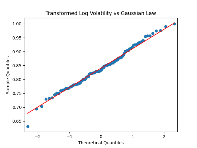
4. Verification. The content of this section is taken from the file vol-transform.py The transformed log volatility is Gaussian, unlike the log volatility before the transformation. The is the parameter for the transformation.
Below we see the quantile-quantile plot of autoregression residuals The regression fit is with Shapiro-Wilk and Jarque-Bera normality tests for give us and respectively.
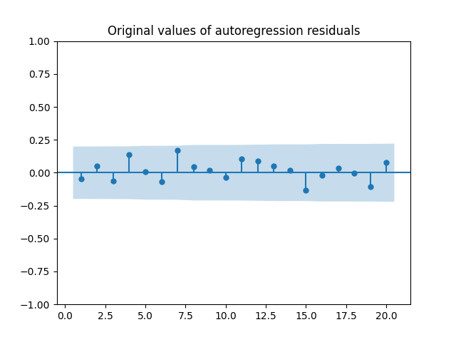
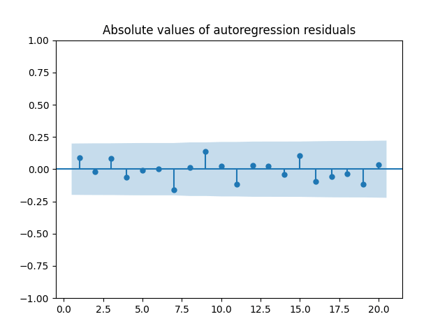
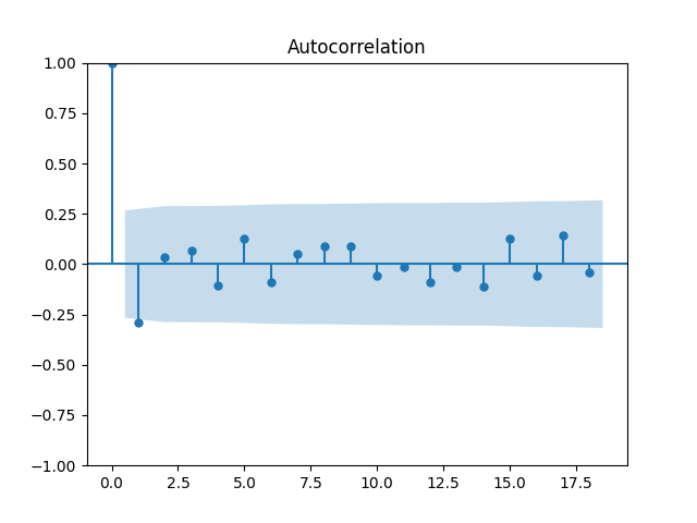
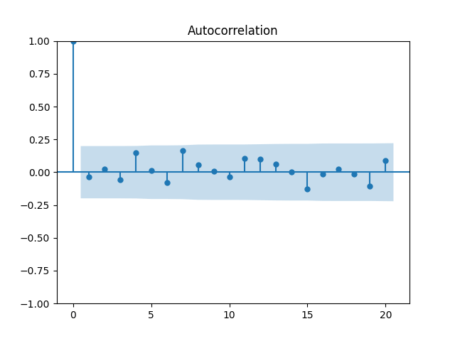
And we see the autocorrelation function for original and absolute values of autoregression innovations. We see that they are well modeled by IID Gaussian random variables.
5. Updates. Apologies, I absolutely forgot that series of the two innovations also need to be correlated. All this was done for two independent series of residuals. But we still benefited from it, since we made this mistake for both original and transformed data; and for classic vs Bayesian. We need to include covariance matrix of innovations, for both classic and Bayesian versions.
Below we provide the three tables for domestic, developed, emerging stocks. Compare them with Section 3.
US stocks, measured by S&P 500, with correlated innovations.
Statistic
Frequentist Original
Bayesian-lite Original
Bayesian-full Original
Frequentist Transformed
Bayesian-lite Transformed
Bayesian-full Transformed
Average
8.1
7.8
7.9
7.7
7.2
7.1
Stdev
4.7
5.7
5.7
5.6
7.5
8.6
Median
8.6
8.6
8.6
8.5
8.4
8.5
10%
2.0
0.5
0.7
0.7
-1.1
-0.9
30%
6.1
5.6
5.7
5.7
5.1
5.3
70%
10.8
11.1
11.1
10.8
11.1
11.1
90%
13.8
14.4
14.4
13.9
14.4
14.4
3% ruin
23
26
25
25
28
27
4% ruin
33
35
34
35
37
36
5% ruin
43
44
44
44
45
45
Developed international markets, measured by 88% MSCI EAFE + 12% MSCI Canada, with correlated innovations.
Statistic
Frequentist Original
Bayesian-lite Original
Bayesian-full Original
Frequentist Transformed
Bayesian-lite Transformed
Bayesian-full Transformed
Average
6.1
5.6
5.6
5.6
4.8
4.6
Stdev
6.1
7.9
8.2
7.2
10.3
16.4
Median
6.7
6.8
6.7
6.6
6.7
6.7
10%
-1.9
-4.5
-4.6
-3.5
-6.6
-6.4
30%
3.4
2.7
2.7
3.0
2.2
2.4
70%
9.6
10.2
10.2
9.7
10.3
10.2
90%
13.3
14.4
14.5
13.5
14.4
14.6
3% survival
39
40
40
40
41
41
4% survival
49
49
49
49
50
49
5% survival
58
58
57
58
57
57
Emerging markets, measured by MSCI EM, with correlated innovations.
Statistic
Frequentist Original
Bayesian-lite Original
Bayesian-full Original
Frequentist Transformed
Bayesian-lite Transformed
Bayesian-full Transformed
Average
6.6
9.05
6.1
5.9
5.1
4.9
Stdev
8.0
5.23
11.0
9.4
13.7
19.3
Median
7.3
9.63
7.6
7.3
7.4
7.4
10%
-3.8
-7.8
-7.8
-5.8
-10.0
-9.8
30%
3.2
2.0
1.9
2.6
1.4
1.6
70%
11.2
12.6
12.4
11.3
12.2
12.3
90%
16.1
18.1
18.2
16.3
18.2
18.4
3% ruin
41
43
42
42
43
44
4% ruin
49
50
49
50
50
50
5% ruin
56
55
55
56
55
56
We see that making residuals correlated makes values at risk for 10% and 30$ even more biased downward, especially for the international markets, where we have less data. Doesn’t it contradict the diversification principle, which states we need to ivnest even in riskier assets, when they are not well correlated with the benchmark? Turns out if there is not enough observations for these risky assets, then this uncertainty in parameter estimates outweighs the variance reduction.
We still need to make changes to our simulator in light of our very recent research:
Replace volatility in the autoregression with its Box-Cox transform. This will model the volatility as the classic autoregression of order 1 with Gaussian IID innovations. Update: we need Yeo-Johnson transform because Box-Cox is valid only for positive values. In this new post, we discussed that Yeo-Johnson transform works for log volatility values, and enables us to apply objective Bayes inference for autoregression coefficients. Update: We did not simulate correlated innovations, as discussed here. We need to correct this.
Edit total returns of 10-year zero-coupon bonds to update equations and account for noise. This will not improve much, but it is important for completeness and intellectual honesty. We will have 9 equations with 9 noise series. Update: we used total returns of 7-year zero-coupon Treasury bonds instead of 10-year zero-coupon Treasury bonds. They fit better because they have IID Gaussian regression residuals without the need of any transforms. And they have more data, going back to 1962.
Update the covariance and the correlation matrix of residuals. They will both be of size 9. Update: We only need the covariance matrix, see item 5 below.
Later we add the following options: Instead of this full version, remove dependence of all three stock returns upon bond duration, valuation measure, and risk spread. Or pick any combination of 3 factors for each stocks. Update: It would be great to code regression fit inside the simulator, otherwise we will need to manually code each and every covariance matrix. This has many shortcomings: (a) It can introduce manual errors. (b) It would take a lot of time. (c) When we change model or data so slightly, even just updating this for one year, we will need to update the entire model, which can lead to (a) or (b). Update: We found, to our shock, there is no loss in runtime. Moreover, 100 or 10000 Monte Carlo simulations? this does not matter for the runtime!
In the above item, check that each version has Gaussian IID residuals, and add Bayesian-full version. Update: We only need the Bayesian-lite version, see item 5 above.
Total 8 versions in item 6, times 2 in item 7, so 16 versions. We could have more options, but let us keep it simple for now. And do not forget to add explicit initial values of the four market factors. Do not write a separate advanced version of the simulator. Fix the current values of these market factors as default ones. But users must see them explicitly and be able to change them.
0. Introduction. Previously, we wrote a deterministic equation connecting the zero-coupon bond rates and the total returns for 10-year bonds. But we only approximated the zero-coupon bond rates with classic 10-year rates, for which we have much more data, back from 1927. And we need zero-coupon bonds to compute exact returns, not classic coupon Treasuries. Here, we explain and address this discrepancy.
1. Why we need zero-coupon bonds.Classic Treasury bonds pay semiannual coupons, so they pay 20 such coupons during their (for example) 10-year lifetime. We choose 10-year bond rates because they have the most data for them, going back to 1927 or even further. There are classic Treasury bonds with other maturities, for example 7-year or 30-year, but their data does not go back enough. Therefore, 10-year Treasury bond rates serve as the classic benchmark for long-term Treasury rates. They are free of default risk, but very much exposed to interest rate risk: If interest rates rise then bond prices fall. This is shown by duration, which is defined as the (minus) partial derivative of the price with respect to the rate. This can be thought of as average time of payments, weighted by the amount of payments (coupons and the principal). Thus we cannot exactly compute returns of such coupon bonds knowing only yield to maturity. We need to know the coupon rate, but usually only yield to maturity is quoted as the rate. This is a solution to a complicated equation which states that if we get coupons and reinvest them at the same rate, then the current price exactly matches all future payments. But this assumes the constant rate, which never happens.
The price (and therefore total returns) is much easier to compute for zero-coupon bonds, which pay only the principal amount. Their maturity, in fact, coincides with their duration. More precisely, if is end-of-year rate for the zero-coupon bond with maturity years and ith continuous compounding, then the price of this bond is One year later, at end of year this becomes a zero-coupon bond with maturity The new price is There are no coupons, therefore price and total returns coincide. The log returns are But where do we get these zero-coupon rates?
2. Data. Previously, it was not great with regard to zero-coupon bond rates data. We had Federal Reserve daily data from January 1990 until now, for maturities 1 year, 2 years, etc up to 10 years. But this is not nearly enough to make inference! Only 36 years. Instead, we found an article in Federal Reserve repository (their own internal version of arXiv or SSRN) which includes data from 1961 for zero-coupon maturities from 1 to 7 years and from 1971 for 8, 9, 10 years.
Target: We compute these log returns using these data for 9-year and 10-year end-of-year zero-coupon bonds, as in the subsection above.
Benchmark: But in addition, we replace and both by which is 10-year December average for year 10-year coupon Treasury rates. And we compute the new version of these log returns. See the GitHub repository where we put our newest version of the simulator with Gaussian innovations. We created a separate subfolder treasury-bonds with data and code files. The data file, as usual, contains detailed description.
We would use the target if we had data for zero-coupon bonds all the way from 1927. But unfortunately, we have them only from 1971. Which is a lot, but not enough. We approximate them by replacing them by the classic 10-year Treasury rate. But of course, this intorduces an error.
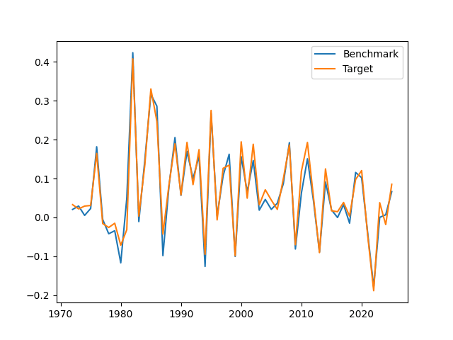
3. Analysis. How to compare these target and benchmark? The correlation is 97.7%. But this masks big differences, as shown in these data files. See the scatterplot and the time series plot below.
Run regression: Target = 0.954 * Benchmark + 0.01 + Residuals with But residuals are not Gaussian.
We tried dividing by volatility and thi did not work. Why such autocorrelation with lag 1? Because this difference is proportional to the long-short term spread (the slope of the Treasury yield curve), but this one has autocorrelation with lag 1, as shown in my current version of the financial simulator.
The Box-Cox transform works: Residuals become Gaussian, but still such a big autocorrelation. Still, lag 1 is the only one, so Ljung-Box white noise test for lags 5 and 10 gives us high p-values, so we fail to reject the IID null hypothesis. The Ljung-Box test for absolute values of residuals also gives us fail to reject.
4. Seven-year zero-coupon Treasury bonds. This turns out to be a better fit. For more years, 1962-2025 (64 years), not 1972-2026 (54 years), you can compute total returns. The above formula in Section 1 works for instead of The correlation is 97.3%, the linear regression is Target = 0.713 * Benchmark + 0.0205 + Residuals. And all tests above give p values above 5%. Thus we really can fit this regression. I will add these total returns for 7-year zero-coupon bonds into my main financial data library. See the Python file in the same subfolder treasury-bonds. We do not need the Box-Cox transform, after all.
0. Introduction. I remembered we can apply the Box-Cox transform to make the data closer to normal. We can do this either with regression inputs, or regression outputs, or regression residuals. The data does not have to be IID. The main goal is to make new regression residuals Gaussian.
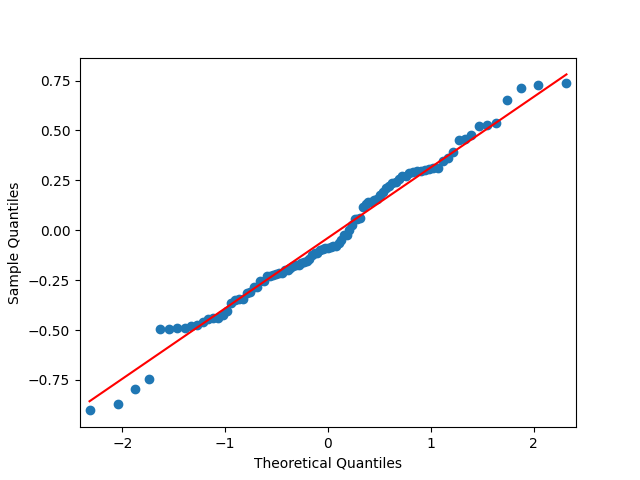
1. The annual volatility. This works very well for annual volatility data, both for raw data and autoregression residuals which are proved to be IID. See the Python code in the same GitHub repository for the current version of the simulator. See the resulting quantile-quantile plots for the transformed volatility; and for the transformed residuals for autoregression of the original log volatility.
See also the autocorrelation function plots for original and absolute values of autoregression residuals for transformed volatility. These are very consistent with being independent identically distributed.
For the Box-Cox transforms of the residuals for the autoregression of original log volatility, we do not need to check that they are independent identically distributed, because we already checked this for these residuals. The normality tests (Shapiro-Wilk and Jarque-Bera) have I think it is better to transform volatility instead of residuals. The index in this Box-Cox transform is -0.594.
2. Other residual series for the current simulator. Consider the non-Gaussian series of residuals from the same repository of the current simulator. They are for Do not forget to exponentiate these residuals, since we need positive data for the Box-Cox transform. The other three regressions have Gaussian residuals, and they are all for asset classes returns. We already discussed the volatility. Judging by the Shapiro-Wilk and Jarque-Bera normality tests, we succeeded in making Gaussian the series for and but failed for and We see this in the file in the same repository.
3. Other data series for the current simulator. Consider the series of data themselves, rather than their residuals: To each apply the Box-Cox transform and then test Gaussianity. We succeed for but fail for Later, fit the autoregression of order 1 to the transformed data, and test innovations for IID Gaussian. We fail for all three series! Such a miserable failure to replicate our results but make them Gaussian. A reminder: We can apply the Box-Cox transform to data for the autoregression and only then fit this autoregression; or to its residuals after fitting the autoregression with original data. Unfortunately, we succeeded only in one case: making Gaussian (and IID) residuals for the BAA rate. This is done in this file in the same repository.
4. Exponentiated total log returns for three asset classes. The data for the Box-Cox transform needs to be positive. This cannot be said for log returns for US stocks, international stocks, and corporate bonds, so we exponentiate each of them. The Box-Cox transform, miraculously, transforms each of them into a sequence of IID Gaussian data. Fantastic! This is also done in the file in the same repository.
But, helpfully, this Box-Cox transform gives us a way out: Just transform the volatility and run the autoregression. This enables us to build a version of our simulator which has indeed only Gaussian innovations. Let us call this Version O.
Another version would be simple, with only asset classes (including maybe emerging stocks, check!) and without volatility at all, the only factor is BAA rate. As discussed above in Section 3, we can transform residuals of the autoregression for log rates to make them Gaussian. Let us call this Version R.
Also, we can include the volatility as in the Version R, and combine this with the BAA rate. This would be Version V.
Finally, we can remove the volatility from the Version O, and apply the Box-Cox transform to these asset class returns. This would be Version C.
None of the versions include long-short spread, and earnings growth. Unfortunately, we cannot transform the current version of the financial simulator into a version with Gaussian innovations.
But we can transform the simple version into the one with Gaussian innovations. This would be Versions R or V. Do not forget to check emerging stocks! Also, we can transform (after checking for emerging stocks!) the newest version, this would be Versions C or O.
6. Stock Returns. I checked log returns of each of three stock asset classes: USA, developed, emerging. For each, I took both the original data and normalized by volatility. For both cases, I took the data itself and after the Box-Cox transform. I applied to each of the resulting 12 series the following tests: Shapiro-Wilk, Jarque-Bera (for normality) and Ljung-Box for 5 and 10 lags for original and absolute values of residuals (for IID).
Outcome: I think it is better to either normalize or transform the returns data, but not both. Better normalize, since this works for all three asset classes. But can we really apply the normality tests on such small sample size, only 1988-2025 (38 data points) for emerging stocks? I am not sure.
US stocks: All pass all tests, except the original (non-normalized and non-transformed) data, which is IID but not Gaussian.
Developed markets: Same as the US stocks.
Emerging markets: All pass all tests, except the Ljung-Box test for original values of 10 lags.
 with unfortunately very low
  .
.  are Gaussian IID, judging by the Ljung-Box test for 5 and 10 lags for
  and
and  and by the Shapiro-Wilk and Jarque-Bera tests.
  but with residuals which are NOT Gaussian IID. Division by volatility does not improve the fit.
  , abbreviated later as VAP) with our
  which we analyze are:
 using Ljung-Box tests for 5 or 10 lags, and we accept IID only if all four tests give us value greater than 5%.
  and we accept Gaussianity only when both tests give us value greater than 5%.
  and apply Steps 2-3 again.
 to
to 
 much like we tested
  and apply Steps 2-3 again.
 and Jarque-Bera
  for transformed log volatility, with
  However, autoregression innovations are IID but not Gaussian, both normality tests give extremely low values.

 and
and  is the inverse Yeo-Johnson transform.
 is Gaussian, unlike the log volatility
  before the transformation. The
  is the parameter for the transformation.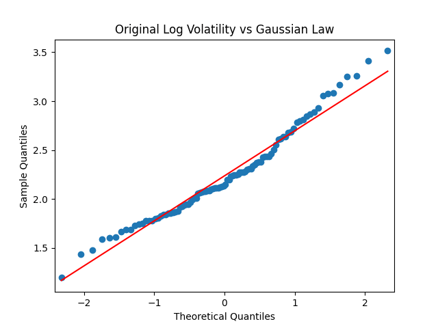
 The regression fit is
  with Shapiro-Wilk and Jarque-Bera normality tests for
  give us
  and
and  respectively.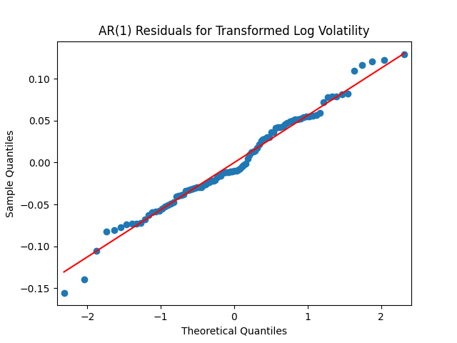
 to the regression of (modified)
  is end-of-year
  rate for the zero-coupon bond with maturity
  years and ith continuous compounding, then the price of this bond is
  One year later, at end of year
  this becomes a zero-coupon bond with maturity
  The new price is
  There are no coupons, therefore price and total returns coincide. The log returns are
  But where do we get these zero-coupon rates?
 and
and  both by
  which is 10-year December average for year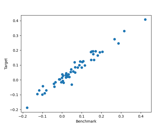
 But residuals are not Gaussian.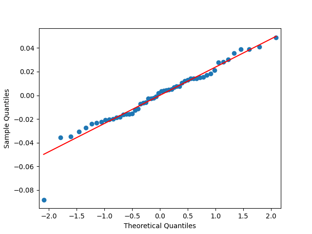
 instead of
  The correlation is 97.3%, the linear regression is Target = 0.713 * Benchmark + 0.0205 + Residuals. And all tests above give p values above 5%. Thus we really can fit this regression. I will add these total returns for 7-year zero-coupon bonds into my main financial data library.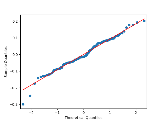
 I think it is better to transform volatility instead of residuals. The index in this Box-Cox transform is -0.594.
  Do not forget to exponentiate these residuals, since we need positive data for the Box-Cox transform. The other three regressions have Gaussian residuals, and they are all for asset classes returns. We already discussed the volatility. Judging by the Shapiro-Wilk and Jarque-Bera normality tests, we succeeded in making Gaussian the series for
  and
and  but failed for
  and
and  We see this
  To each apply the Box-Cox transform and then test Gaussianity. We succeed for
  but fail for
  Later, fit the autoregression of order 1 to the transformed data, and test innovations for IID Gaussian. We fail for all three series! Such a miserable failure to replicate our results but make them Gaussian. A reminder: We can apply the Box-Cox transform to data for the autoregression and only then fit this autoregression; or to its residuals after fitting the autoregression with original data. Unfortunately, we succeeded only in one case: making Gaussian (and IID) residuals for the BAA rate. This is done


