This work was done by my undergraduate student Ian Anderson, using the volatility data computed by my other undergraduate student Angel Piotrowski, see the previous post.
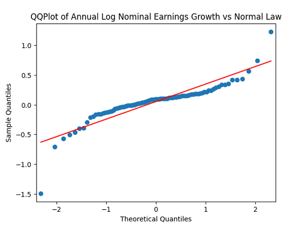
Ian took 1927-2023 net earnings of Standard & Poor 500 (since 1957; or its predecessor Standard & Poor 90) and compute annual growth We do this first for nominal earnings, without adjustment for inflation. We analyze whether it is Gaussian independent identically distributed. We make the quantile-quantile (QQ) plot versus the normal distribution.
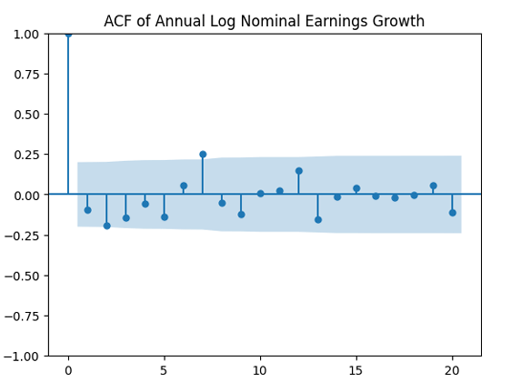
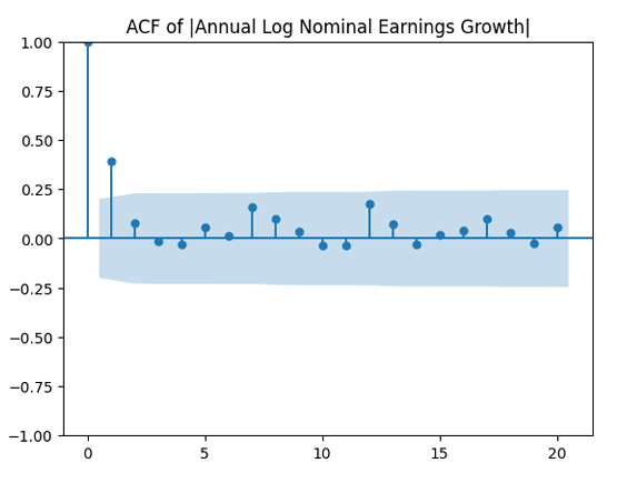
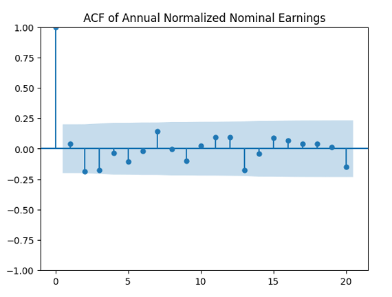
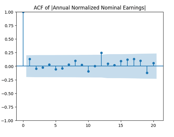
And we plot the autocorrelation function for and another plot for the autocorrelation function for
We see from the QQ plot that, unfortunately, earnings growth terms are not Gaussian. The autocorrelation function for earnings growth corresponds to white noise: It shows that and are uncorrelated. But with absolute values, this is not true. There is a significant autocorrelation of lag 1:
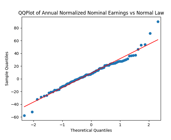
Then divide the earnings growth by annual volatility and get Does this division improve these terms to make them closer to Gaussian independent identically distributed? In fact, yes!
We see that now both autocorrelation plots show lack of significant autocorrelations. And the quantile-quantile plot is much closer to linear. Thus it makes sense to model as independent identically distributed Gaussian.
The same happens if we consider real earnings (inflation-adjusted) instead of nominal earnings, using December data for the Consumer Price Index. Thus we have joint model for earnings and volatility, annual 1927-2023:
are independent identically distributed bivariate normal, with mean zero and covariance 2×2 matrix This works for both nominal and real annual earnings, but not for dividends.
Consider the spread between 10-year Treasury rate and 1-year Treasury rate. Usually, long-term rates are higher than short-term rates, since investors want extra compensation for committing their money for a long time. Another way to express this is that long-term bonds are more exposed to interest rate risk: If bond rates rise then bond prices fall. The coefficient is called the duration, and it is higher for long-term bonds.
But sometimes, long-term rates are lower than short-term rates. This is usually not a good sign, and a harbinger of a recession. Expecting a recession soon, investors anticipate short-term interest rate cuts by the Federal Reserve. This influences current long-term rates, which incorporate current and expected future short-term rates.
Denote this spread by Apply an autoregression of order 1: We expect mean reversion for this spread, which is true for This is different from where this process is a random walk, when future movements are independent of the past.
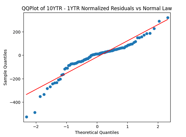
Let us now analyze the innovations, otherwise called regression residuals: Apply the quantile-quantile plot versus the normal distribution. Next, divide these innovations by annual volatility and make the quantile-quantile plot again.
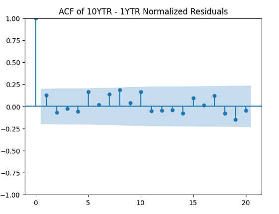
We do not see much difference… Does not seem to be normal. But let us apply the autocorrelation function to these innovations Next, divide by the volatility and plot the autocorrelation function again, now for Both plots seem to be for white noise, no autocorrelation.
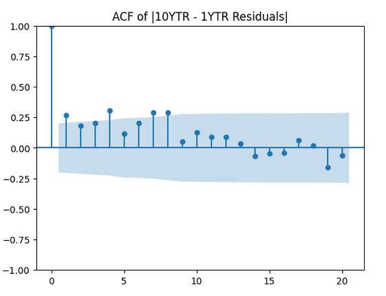
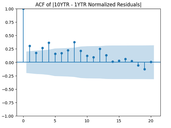
Finally, apply the autocorrelation function to the absolute value and see whether it is truly independent? It is not. Next, divide by volatility and apply the autocorrelation function to to see whether it improves the result. It does not, in fact!
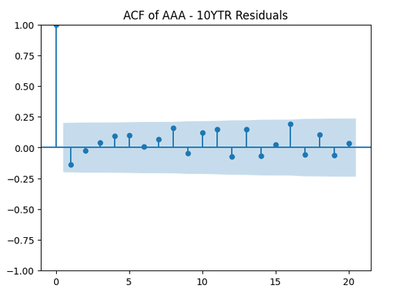
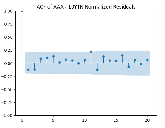
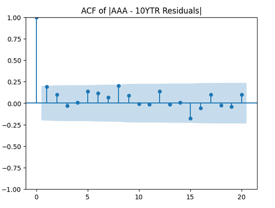
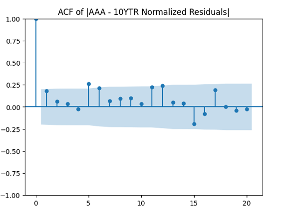
But now let us fit the same for the bond spread between AAA Moody’s rate and 10-year Treasury rate. The AAA rating is the highest reserved for corporate and municipal bonds, which have the lowest default risk.
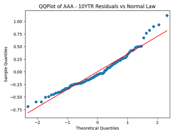
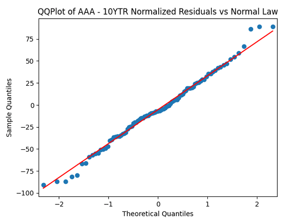
QQ plot of innovations before normalization, close to normal but not quite. QQ plot of innovations after normalizations: Much closer to normal!
Autocorrelation function for innovations before and after normalizing: Good!
Autocorrelation function for absolute values of innovations before and after normalizing: Not so good, but acceptable. We need some further white noise testing.
The AAA-1YTR spread results are the same as for 10YTR-1YTR. Here TR stands for Treasury Rate.
Thus, the answer to the question in the title: Using volatility improves autoregression of order 1 for credit risk spread AAA-10YTR but not for long-short term spread 10YTR-1YTR and not for combined spread AAA-1YTR.


![(W(t), Z(t)) \sim \mathcal N_2([0, 0], \Sigma)](https://s0.wp.com/latex.php?latex=+%28W%28t%29%2C+Z%28t%29%29+%5Csim+%5Cmathcal+N_2%28%5B0%2C+0%5D%2C+%5CSigma%29+&bg=ffffff&fg=000&s=0&c=20201002)

 Apply an autoregression of order 1:
  We expect mean reversion for this spread, which is true for
  This is different from
  where this process is a random walk, when future movements are independent of the past.
  Apply the quantile-quantile plot versus the normal distribution. Next, divide these innovations by annual volatility and make the quantile-quantile plot again.
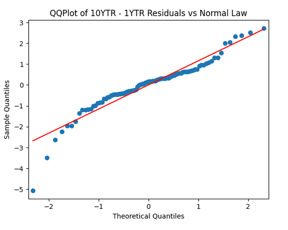
 Next, divide by the volatility and plot the autocorrelation function again, now for
  Both plots seem to be for white noise, no autocorrelation.
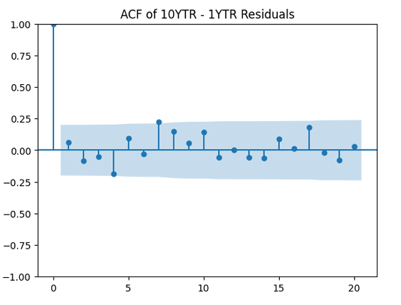
 and see whether it is truly independent? It is not. Next, divide by volatility and apply the autocorrelation function to
  to see whether it improves the result. It does not, in fact!