Model explanation: Continuing research by Ian Anderson with updated data, 1927-2024, consider the following model for and which are spreads BAA-AAA and BAA-Long. Here, AAA and BAA are Moody’s December daily average rates, and Long is 10-year Treasury December daily average rates. In the previous post, we discussed that these are well-modeled as a vector autoregression of order 1, with mean reversion in the long run, if only we divide innovations and by annual volatility, computed by my other undergraduate student Angel Piotrowski. Then are independent identically distributed bivariate Gaussian.
As usual, this can unfortunately lead to ordinary least squares for regression fitting not applicable. Let us first divide each question by annual volatility, and add an intercept (constant) for completeness (because usually, linear regression includes an intercept). We get:
In the vector form, we can write this as
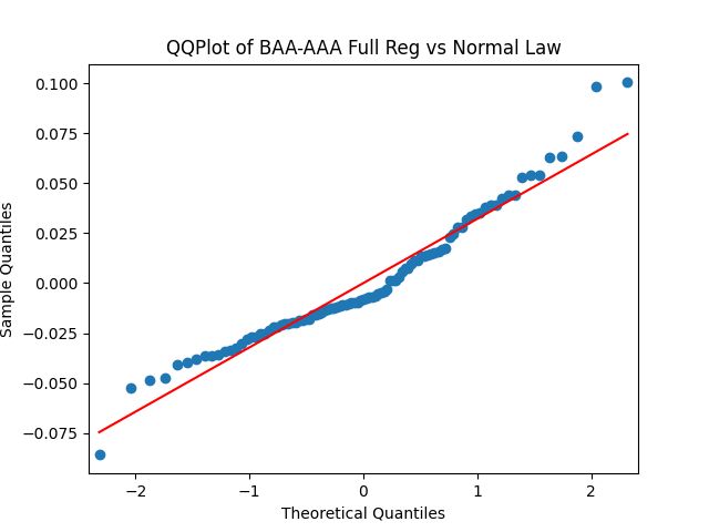
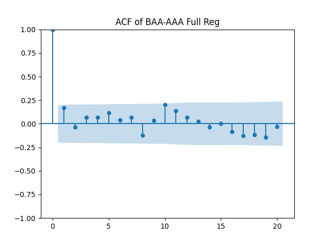
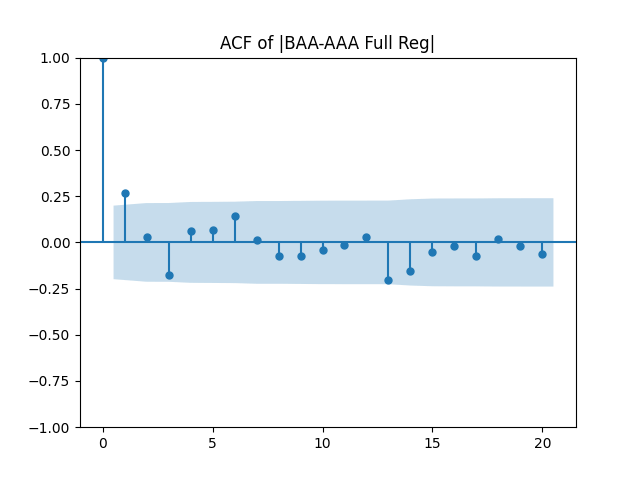
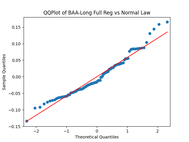
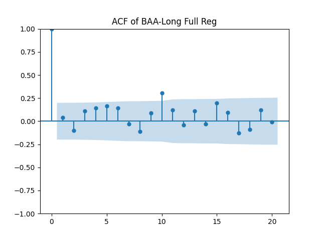
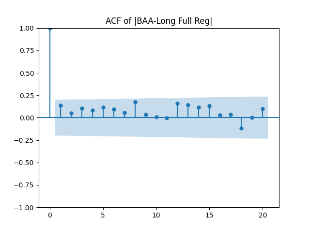
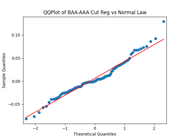
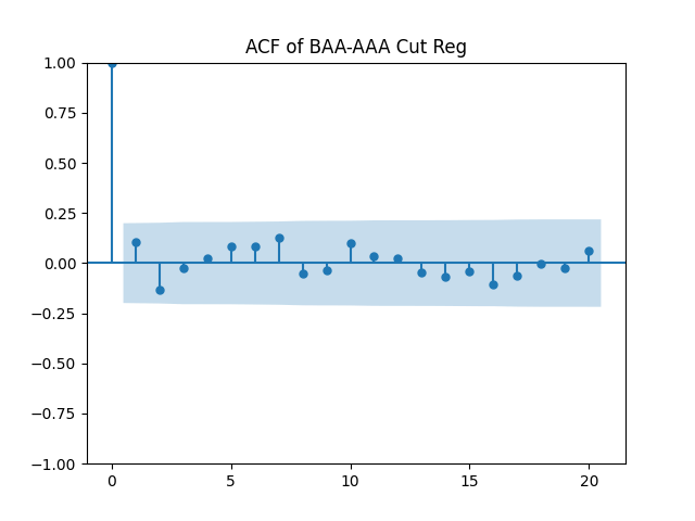
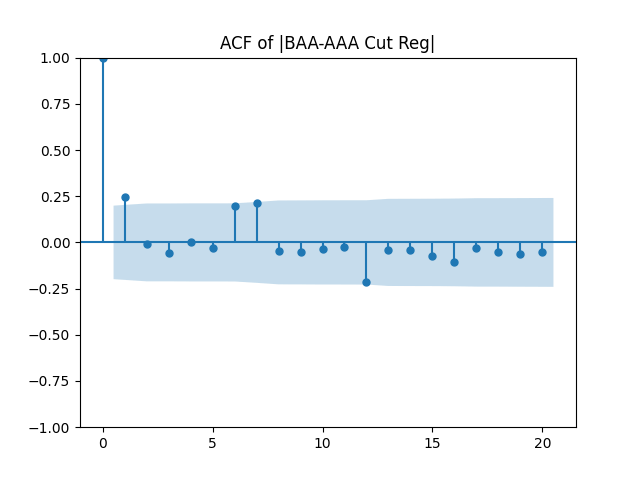
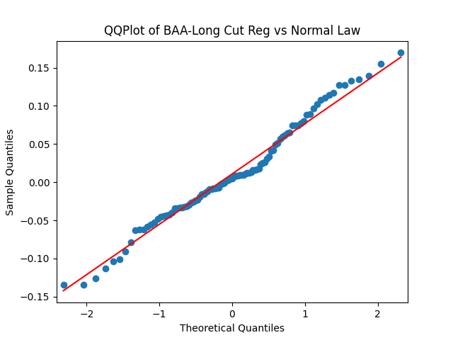
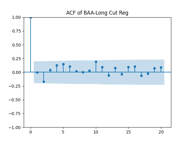
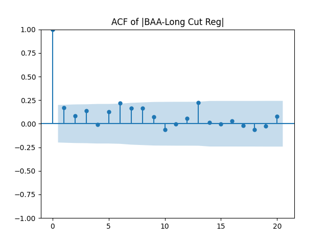
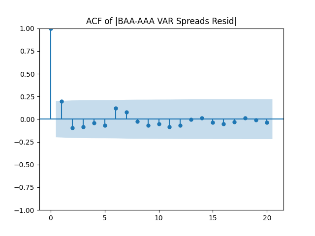
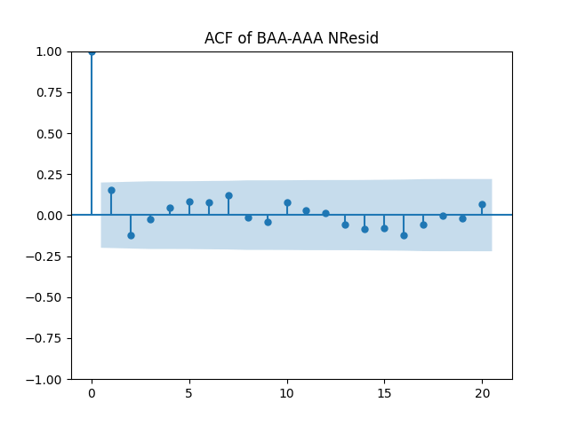
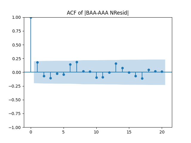
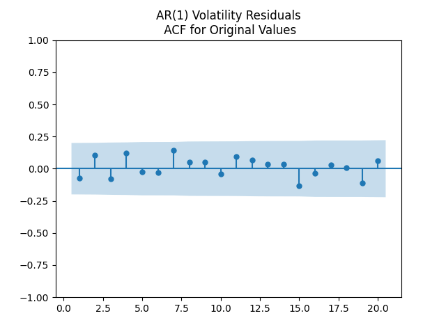
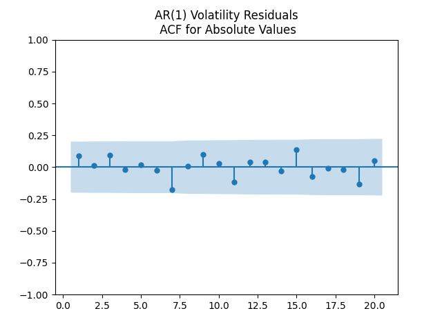
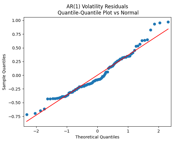
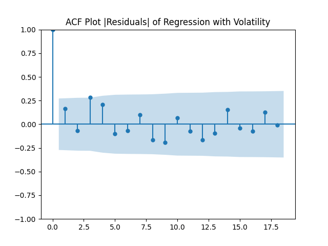
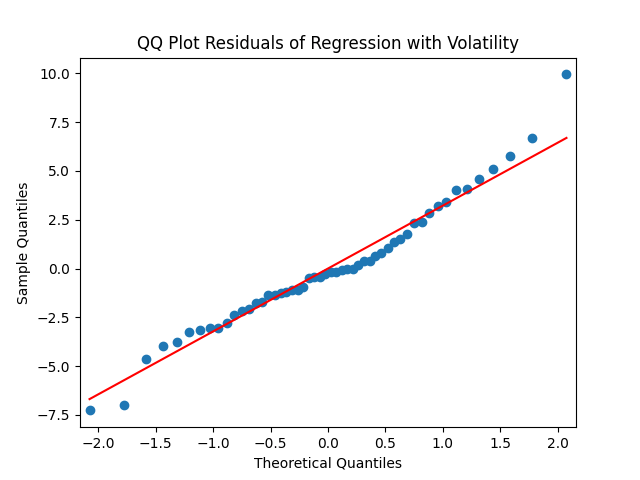
Results: Unfortunately, innovations here are further from Gaussian than in the previous post. Judging by the autocorrelation function plots for these innovations and for their absolute values: Yes, we can model as independent identically distributed. Same is shown by the L1 norms. But the quantile-quantile plots clearly say these are not Gaussian. Similarly, the Shapiro-Wilk and Jarque-Bera tests give us very low p-values.
Innovations
Skewness (Gaussian = 0)
Kurtosis (Gaussian = 0)
Shapiro-Wilk p-value
Jarque-Bera p-value
L1 norm for 5 lags ACF of original values
L1 norm for 5 lags ACF of absolute values
BAA-AAA
0.714
0.847
0.2%
0.4%
0.45
0.605
BAA-Long
0.631
0.181
1.0%
3.7%
0.554
0.487
We recall that the threshold 95% value for the L1 statistic is around 63%, based on Monte Carlo simulations.
Dependence upon volatility which corresponds to the term is positive and very significant. The Student T-test gives us For both regressions,
Removing intercepts: If we do the vector model above without , we get much improved innovation sequences. Compare L1 norm values:
Innovations
Skewness (Gaussian = 0)
Kurtosis (Gaussian = 0)
Shapiro-Wilk p-value
Jarque-Bera p-value
L1 norm for 5 lags ACF of original values
L1 norm for 5 lags ACF of absolute values
BAA-AAA
0.5
0.819
2.8%
3.4%
0.375
0.342
BAA-Long
0.204
-0.203
15.9%
65.8%
0.489
0.528
The p-values for Student T-test for BAA-AAA with factor BAA-Long is 32.3% and the other way around is 43%. In principle, we could model these two spreads as separate autoregressions of order 1, but with correlated innovations.
Conclusion: For bivariate vector autoregression of order 1 applied to BAA-AAA and BAA-Long spreads, dividing innovations by volatility makes them independent identically distributed Gaussian. After that, adding this volatility as a factor in a linear regression improves the fit as judging by significant dependence, and keeps innovations independent identically distributed, but destroys their normality.
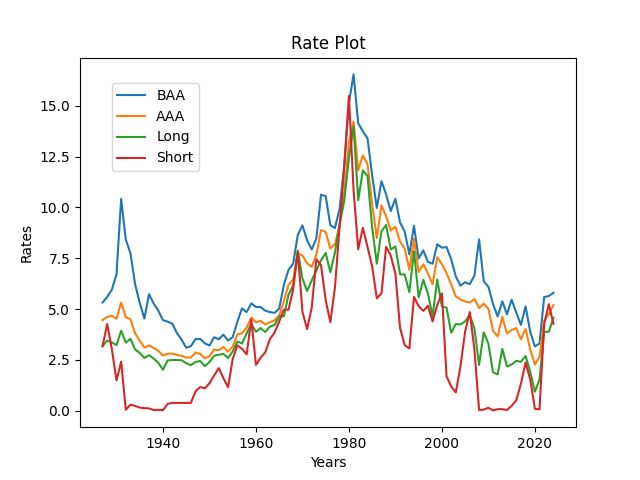
Data description: This research is an improvement of Ian Anderson’s research. See GitHub/asarantsev repository 4rates, which contains Python code, Excel data, and all generated pictures. We take four series of USA bond rates, annual end-of-year (December, monthly average) data:
Short: 3-6 month government yields 1927-1933, 3-month 1934-now
Long: long-term government yields 1927-1963, 10-year 1964-now
AAA Moody’s
BAA Moody’s
We need to take this because this is an improvement over existing Robert Shiller’s data: Hard to find long and short-term interest rates. Also, Robert Shiller’s data is average January, and our data is December. But to model next year’s stock returns, we need the data we know by the end of this year: Thus we need December, not January.
Statistical Methodology: For each series, we fit an autoregression of order 1: We analyze innovations for Gaussian IID. Next, we divide for annual volatility available for 1928-2024, and analyze for Gaussian IID.
Analysis for Gaussian IID is performed as follows:
Skewness (with Gaussian = 0)
Kurtosis (with Gaussian = 0)
Shapiro-Wilk normality test
Jarque-Bera normality test
Quantile-quantile plot versus the normal distribution
L1 norm for autocorrelation function for original values, 5 lags
L1 norm for autocorrelation function for absolute values, 5 lags
Autocorrelation function plot for original values
Autocorrelation function plot for absolute values
For items 1, 2, 6, 7, we use the Monte Carlo simulations giving us 95% and 99% percentiles. This allows us to make normality tests and white noise tests.
Analysis of rates: We summarize results in the table below. The sign XXXXX shows we have independent identically distributed Gaussian innovations. If we have only one of two features: Gaussian but not independent identically distributed, or vice versa, we show it. The term Success means Independent identically distributed Gaussian.
Rate
Original innovations
Normalized innovations
BAA
Independent identically distributed
XXXXX
AAA
XXXXX
XXXXX
Long
XXXXX
XXXXX
Short
XXXXX
XXXXX
Thus we can use autoregression only for BAA rates: Here the for the Student T-test. Here are independent identically distributed but not Gaussian.
Also, we apply the vector autoregression of order 1 for the vector of all four rates. Then we apply the same analysis to each of the four series of innovations. Unfortunately but not surprising, we have complete failure for all innovations. First, we present the autocorrelation and cross-correlation function plots for these four series.
Seems like all plots correspond to white noise. But plots of absolute values of innovations show our failure. We summarize:
Rate
Original innovations
Normalized innovations
BAA
Independent identically distributed
Independent identically distributed
AAA
XXXXX
XXXXX
Long
Gaussian
XXXXX
Short
XXXXX
XXXXX
Bond spreads: Finally, we do the same analysis for spreads. There are six series of spreads.
Spread
Original innovations
Normalized innovations
BAA-AAA
Independent identically distributed
Success
AAA-Long
Independent identically distributed
Gaussian
Long-Short
Independent identically distributed
XXXXX
BAA-Long
Independent identically distributed
Success
BAA-Short
Independent identically distributed
XXXXX
AAA-Short
XXXXX
XXXXX
Let us write autoregression for BAA-AAA, AAA-Long and BAA-Long (all Student p-values are very small):
BAA-AAA: and
AAA-Long: and
BAA-Long and
Vector autoregression for two spreads BAA-AAA, BAA-Long: We write vector autoregression for bivariate series which is BAA-AAA, BAA-Long:
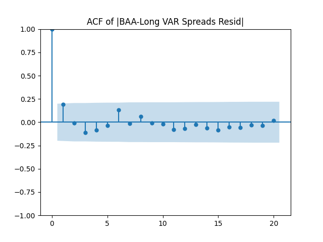
Overall, it seems reasonable for us to model as independent identically distributed. See below the autocorrelation and cross-correlation plots. The correlation of its two components is 89%.
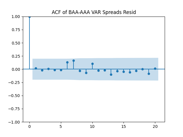
Below see plots for the first series of residuals before normalization: the quantile-quantile plot versus the normal distribution; the autocorrelation function for ; the autocorrelation function for We see it is reasonable to model as independent identically distributed but not Gaussian.
Next, we normalize these residuals by dividing them by and make the three plots for We see it is reasonable to model as independent identically distributed normal.
Similar results are true for . Make the three plots for this second series of residuals.
And make the same plots after division by
Conclusion. We can model [BAA-AAA, BAA-Long] as bivariate mean-reverting vector autoregression of order 1 with bivariate Gaussian innovations. All other rates and spreads do not allow autoregression modeling with Gaussian innovations.
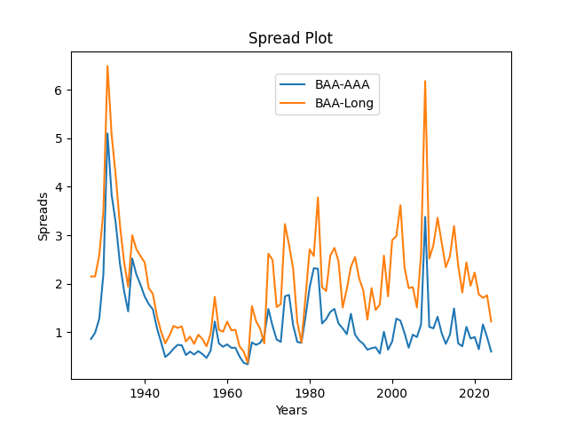
Of course, the spread between BAA rates and AAA rates is smaller than between BAA rates and long-term Treasury rates.
I wrote about this manuscript in a previous post. It was returned for review after two years. This is a very long time.
I updated it with new data from 2023 and 2024, corrected some misprints, and returned it to editors and reviewers for further review. I hope it gets published soon.
Luckily, this new data did not change any of my conclusions:
This new valuation measure takes into account the difference between total returns and fundamentals growth.
This measure works best if we take trailing averaged earnings: Innovations for the autoregressions are independent identically distributed and Gaussian.
We have annual volatility and earnings as two factors, as in the previous post. We here use trailing averaged annual earnings over a few years instead of earnings over the last year. This averaging time window ranges from 2 to 10 years. This is similar to the 10-year trailing averaged earnings used in the Shiller cyclically adjusted price-earnings ratio. The inverse of a price-earnings ratio is called earnings yield.
Model: The equations from the previous post stay the same. We model earnings growth normalized by volatility for 1-year earnings. But for the returns, regression has trailing averaged earnings. The data are the same: earnings and inflation for 1927-2024, returns and volatility for 1928-2024. But we add a few data points for earnings and inflation for years 1918-1926. Indeed, we need to compute 10-year averaged earnings, and thus we need a few more trailing data. The data is from my web site.
We take real and nominal earnings and returns. We have 4 types of returns: nominal total, nominal price, real total, real price.
Modification: But then we have a problem with initial conditions. Assume we take a 10-year window. To get earnings yield for year we need earnings from years To get earnings yield for year we need earnings from years And so on for subsequent years. Thus we need all earnings for each of the last 10 years to be able to simulate returns from this year.
It is not enough to provide only earnings for the last year, or averaged earnings over the last 10 years. These initial conditions would not be sufficient to perform the simulation. We think it would be hard for a user to provide all earnings for each of these 10 years.
Thus I made the following decision. I simply removed the option of choosing initial earnings. The simulator always uses the earnings for the actual last 10 years. The same is true for volatility. We start the simulation from the actual year 2025.
Results for 10-year window: Dependence of returns upon earnings yields is much stronger than in the previous post: for all four types of returns. Thus we might state that the 10-year averaging improves the model. However, the values are of the same order: around 20-30%.
Residuals for regressions of returns are normal. Autocorrelation function plots seem better, although still with a strange spike at lag 4.
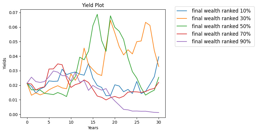
Simulations show the earnings yield can fluctuate but not nearly as wildly as in the previous post. The picked simulations have yields less than 7%. See the plot below.
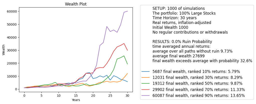
Finally, the wealth simulation fluctuates much less. We try 30 years time horizon without any withdrawals or contributions. Overall average returns are more reasonable 9.63%. More importantly, the 90% quantile of average total returns is only 13.65%, much less extreme than in the previous post.
Conclusions: We think the Shiller CAPE, or, equivalently, cyclically adjusted earnings yield with 10 years of averaging window works much better than the annual price-earnings ratio, or equivalently, annual earnings yield. We added annual volatility to the classic Campbell and Shiller’s research and much improved it. Now we have a dynamic stochastic general equilibrium (DSGE) model: We can simulate it for each time step; It is stable in the long run; and it has Gaussian IID innovations.
In the previous blog post, I have written about the simulator using only one factor: annual volatility, and two equations: for volatility and for total returns. Annual volatility was computed by my undergraduate student Angel Piotrowski as realized standard deviation of daily price returns. I multiplied it by 1000 for normalizing.
Our Model: Here, I extended it to two factors: annual volatility and annual earnings. Previously, annual earnings growth was modeled by another undergraduate student Ian Anderson. We have four equations:
Autoregression of order 1 for logarithmic volatility
Earnings growth divided by volatility as IID
Price returns (excluding dividends) as linear regression with innovations = IID times volatility
Total returns (including dividends) as linear regression with innovations = IID times volatility
These two regressions have factors: this year’s volatility and previous year’s earnings yield: last year’s earnings divided by end of last year’s index. This earnings yield is the classic valuation measure used by financial practitioners.
This model has two versions for the last three equations: nominal (not inflation-adjusted) and real (inflation-adjusted). We use four series of innovations which are multivariate Gaussian: with mean zero. Let us write these equations explicitly. Let and be earnings and volatility in year Let be the end of year index level. Let be total returns for this index, including dividends. Then we have:
Volatility:
Earnings growth:
Price returns:
Total returns:
Regression Results: Below is the table. We see that coefficients are significantly different from zero. In particular, returns and volatility have significant negative dependence. But is not significantly different from zero. Interestingly, we see that dependence of returns upon earnings yield is positive (undervalued markets grow faster) but very weak. A better measure might be cyclically adjusted price-earnings ratio, called Shiller CAPE, see future posts. This ratio is based on 10-year trailing averaged inflation-adjusted earnings.
Presumably this low prediction value is because of high volatility of earnings. For example, in 2008 earnings plummeted so much that the yield plummeted as well, thus making the markets seem overvalued. But in reality, they were undervalued, since earnings rebounded fast, and it took the markets an entire decade to rebound.
Point Estimate
95% Confidence Interval
p-value for Student test
Real Returns
0.1655
[0.064, 0.267]
0.002
Real Returns
-0.0141
[-0.024, -0.005]
0.004
Real Returns
0.1453
[-0.903, 1.194]
0.784
Real Returns
0.1668
[0.068, 0.265]
0.001
Real Returns
-0.0136
[-0.023, -0.004]
0.004
Real Returns
0.5494
[-0.465, 1.564]
0.285
Nominal Returns
0.1693
[0.074, 0.264]
0.001
Nominal Returns
-0.0133
[-0.022, -0.004]
0.003
Nominal Returns
0.4432
[-0.537, 1.424]
0.372
Nominal Returns
0.1706
[0.079, 0.262]
0.000
Nominal Returns
-0.0127
[-0.021, -0.004]
0.004
Nominal Returns
0.8473
[-0.097, 1.792]
0.078
Normality: Skewness, kurtosis, and normality tests (Shapiro-Wilk and Jarque-Bera) show that residuals for price and total returns are Gaussian. However, evidence for normality of earnings growth normalized by volatility; or, equivalently, residuals The Shapiro-Wilk tests for nominal and real earnings growth give us which are 4.6% and 5.8%. The Jarque-Bera tests give us 0.2% and 0.5%. Kurtosis is especially large: 4.7 for nominal and 4.5 for real versus 3 for Gaussian.
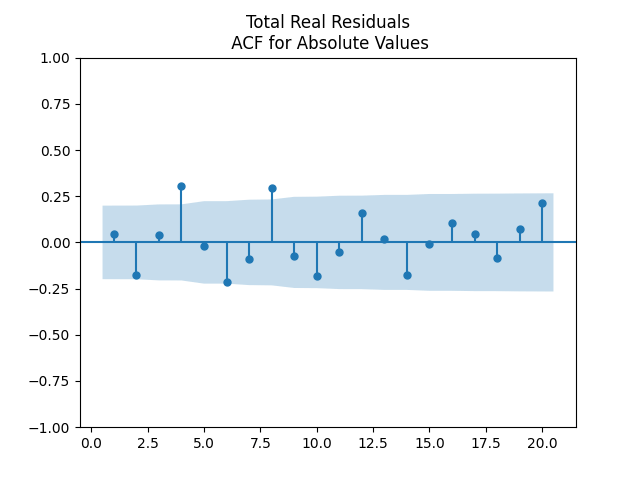
Independence: We show below the autocorrelation functions for original values of residuals: and We pick the regression for total real returns. Evidence for IID is there but there are problems with this. We are not sure why there is large autocorrelation with lag 4. We did not apply the Ljung-Box omnibus test for the first 5 or 10 autocorrelation values. But we think it would reject the white noise hypothesis. Other regressions for other returns: price real, total nominal, price nominal, show similar autocorrelation plots for residuals and their absolute values.
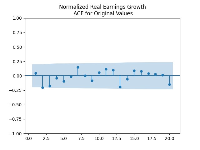
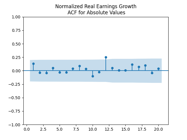
Next, the autocorrelation function plots for nominal and real growth terms show that these can indeed be modeled by IID. We show plots for real earnings growth. Nominal earnings growth have similar autocorrelation plots.
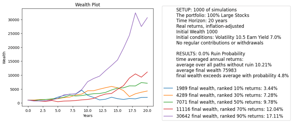
Simulation. We built a version of the financial simulator which has inputs: initial volatility, initial earnings yield, and time horizon in years. We also allow, as usual, annual contributions or withdrawals. We allow for nominal (not inflation-adjusted) or real (inflation-adjusted) versions. The code and data are available on GitHub/asarantsev repository earnings-yield-annual-simulator. We see the graph of total wealth below. This graph also shows:
No contributions or withdrawals
Real returns
20 years time horizon
Initial volatility: 10.5 (close to historical average)
Initial earnings yield: 7% (close to historical average)
We see that average returns over time and all simulations is 10.21%. This is much higher than historical average returns: 6.7%. This presents a problem: If we start with average data, then we should reproduce historical average returns over many simulations. We also see that with high probability returns are very large: the 90% quantile is 17.11%.
Finally, plot earnings yields for the five chosen simulations. We see that yields can become very high. In two simulations out of five, we have yields greater than 30%. Yields like this do not happen in real life.
What is the reason? We think it is because we have exponential terms in the time series equation for earnings yield Note that the log change in earnings yield can be represented as the difference between price returns and earnings growth:
Take the equations for earnings growth and price returns at the beginning of this post. Plug them into the above equation:
The change in depends on exponentially. This might lead to volatile fluctuations, especially when the yield is large. Then fluctuations are also large. This needs to be researched further.
Conclusion: We think this makes our research financially unrealistic, despite rigorous statistical analysis. A better way might be to use the CAPE or its inverse, cyclically adjusted earnings yield (using the last few years average for earnings instead of only last year). Another way might be to reproduce my research on the new valuation measure.
Here, we can model as IID, judging by the ACF plot for and the ACF plot for
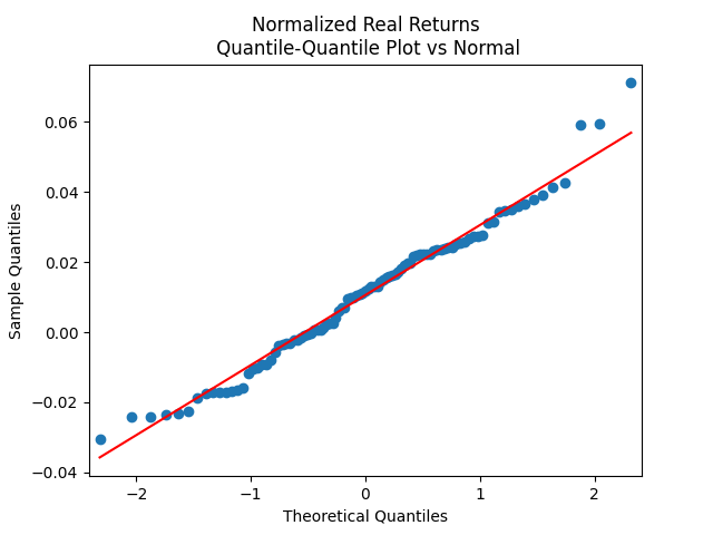
It turns out we cannot quite model by a normal distribution. But it is quite close. See also the table below. This is quite weak evidence of normality! Next, we model total (including dividends) real (inflation-adjusted) returns as follows: for IID Gaussian:
These normalized returns are very well modeled by IID Gaussian. This is confirmed by the plots above. Similar plots are found for the nominal versions of returns.
Data
Skewness (normal =0)
Kurtosis (normal = 0)
Shapiro-Wilk
Jarque-Bera
AR(1) Innovations for Log Volatility
0.59
0.057
0.94%
6.1%
Normalized Total Nominal Returns
0.22
-0.21
11%
60%
Normalized Total Real Returns
0.24
0.023
20%
63%
We model as bivariate normal IID: We found the mean vector and the covariance matrix, for both real and nominal versions. This is available when we run the code.
Next, the code has a function which simulates 1000 paths of wealth:
for This formula would be true for the case when there are no contributions or withdrawals. If each year we have flow (inflow or outflow) (positive or negative), then the wealth process is
The arguments of this function are:
Choose: Real or Nominal?
initial wealth
flow each year
time horizon in years
initial volatility
We rank 1000 simulations by final wealth. This is the same ranking as by average total returns, if only we have no contributions or withdrawals. But if we do have inflows or outflows every year, then these rankings by wealth vs by returns might be different. For each paths, we compute average total returns
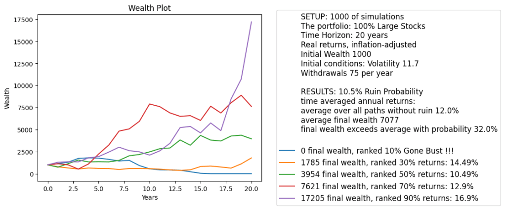
We pick simulations corresponding to 10%, 30%, 50%, 70%, 90% ranking of final wealth. We chose these because it gives us more or less comprehensive picture of randomness. It is trivial but often neglected that markets have a lot of volatility. It is not enough to provide mean or median returns or wealth. We need the entire distribution.
One could suggest a histogram of final wealth. But a histogram is hard to read by ordinary users. Also, it shows less information than wealth paths. To laypeople, wealth paths fluctuate wildly, and the path which are on top now can drop fast later. But the histogram does not show that.
Why choose these 5 quantiles? We need to show the median (typical wealth) and the outliers. But one should not go too far. Showing the path corresponding to the maximal or minimal final wealth would give a distorted picture: Users might misunderstand these and think that such outcomes are typical. Even showing the paths corresponding to 5% or 95% final wealth are not very typical: These are outliers, atypical outcomes.
The range of 10%, 30%, 50%, 70%, 90% shows full range of outcomes, but only typical outcomes, not outliers.
We also stress that average final wealth does not mean we exceed this wealth in 50% of simulations. The distribution of the final wealth is much skewed, so mean and median are not the same!
Note than in case of withdrawals, the path might end in ruin (bankruptcy; zero wealth). If some of the chosen five paths has this, we show this and we do not compute average total returns. We also compute average total returns for paths which do not end up in ruin.
We compute how many paths end in ruin, thus the empirical probability of ruin. This is a major problem in retirement planning: How much can we withdraw per year so that we do not end up in ruin? The classic withdrawal rate is 4% (of initial wealth) per year, if we adjust these withdrawals for inflation.
We adapted the Python code for running locally, so it contains a function which makes this plot below. This is quite different from the Python code in the simulator, which includes entering data from a web page and putting the output using this web page. We also have HTML code for this web page. For running this Python code locally, obviously we do not need this HTML page, only the Python code itself.
Interestingly, even gigantic 7.5% annual withdrawal rate within 20 years results in only 10.5% ruin probability! Our analysis shows we can be much more permissive with withdrawals than the classic 4% rule.
This is statistical description for the Financial Simulator built using Python Anywhere.
Idea: We divide large and small stock returns by volatility, which makes them closer to normal and independent identically distributed (IID). This is Chicago Board of Exchange Volatility Index (VIX), available from 1986. After division by VIX, large stock returns become IID normal. See the code and data at a GitHub repository.
Data: Try January 1986 – May 2024, time points, except for volatility, which has data points. It is taken from Federal Reserve Economic Data (FRED) web site from time series VXOCLS (monthly average data: Jan 1986 – Feb 1990) and VIXCLS (monthly average data: Mar 1990 – Jun 2024):
Large and small stock returns are from Kenneth French Data Library (Portfolios Formed on Size): for large stocks (measured by top 30%); and for small stocks (measured by middle 40%). These are nominal (not inflation adjusted). To adjust them for inflation, we need to subtract monthly inflation rate, computed from the (not seasonally adjusted) Consumer Price Index taken from FRED. We get then real (inflation-adjusted) versions of returns. We also use short (3-month) and long (10-year) Treasury rates from FRED: end-of-month data Dec 1985 – Jun 2024. We are interested in long-short spread:
Modeling volatility: We model VIX as autoregression of order 1 in the logarithmic scale:
where are independent identically distributed innovations with mean zero. This is a mean-reverting process, stable in the long run. e model residuals as follows: Remove 12 outliers from the 461 in the right tail and model the rest as normal with mean and standard deviation and Thus innovations are modeled as a mixture with weights of the uniform distribution upon these 12 outliers, and the above normal distribution. We use kernel density estimation to simulate innovations, with Gaussian kernel and bandwidth derived from the Silverman rule of thumb. In this case the bandwidth is 0.03619. This follows the old blog post.
Modeling long-short bond spread: We model spread as autoregression of order 1 but with additional volatility factor, with residuals normalized by volatility:
This is similar to Ian Anderson’s work but for monthly instead of annual data, and from 1986 instead of 1928.
Modeling stock returns: For nominal returns, we model large and small returns as
For real returns, we model large and small returns as
My undergraduate student Ian Anderson did this research available on his GitHub repository. He continued his research on earnings growth from the previous post. In that research, Ian considers growth terms where are earnings during year These earnings might be nominal (not inflation-adjusted) or real (inflation-adjusted). These are NOT IID Gaussian.
Enter the annual realized volatility computed by another undergraduate student Angel Piotrowski. Denote it by and divide by it the growth terms. These normalized earnings growth terms are, in fact, IID Gaussian.
But are they dependent upon bond rates or spreads? Ian ran simple linear regression of upon where we take rate data for January of year He has data 1928-2023. All regression residuals have ACF and QQ plots which show they can be modeled by IID Gaussian. Not surprising since terms are also IID Gaussian. Results for real (inflation-adjusted) earnings are given below.
Quantity
AAA Corporate Rate
10 Year Treasury Rate
1 Year Treasury Rate
AAA – 10YTR Spread
Slope estimate
-1.06
-1.33
-1.36
7.40
Slope p-value
20%
11%
4%
8%
Intercept estimate
10.95
11.33
10.38
-1.46
Intercept p-value
4%
1%
0%
73%
Correlation r
-13%
-17%
-22%
18%
We see that the correlation is significant for 1 year Treasury rate and (to a less extent) for the spread.
It is easy to explain the first correlation: Lower short-term rates make borrowing cheaper and increase access to capital, so earnings grow faster.
What about the second correlation? Such spread is larger in periods of turbulence, with risk premium increasing. But it is not clear why the correlation must be positive.
Results for nominal earnings growth are not very different, except in this case no correlation is strong enough to be statistically significant. The strongest correlation is again with 1-year Treasury rate, which is -14%, and the p-value (the smallest among the four) is 16%.
In the two previous blog posts, we considered rates and returns for Bank of America-rated corporate bond portfolios, with ratings AAA, AA, A, BBB, BB, B, CCC. We analyzed annual data and used annual averaged VIX (S&P 500 volatility index) to fit Markov time series models. We were successful: For 5 of these 7 ratings, we created a trivariate model with independent identically distributed trivariate Gaussian innovations. Unfortunately, data was available only starting from 1996. This is less than 30 years.
It would be nice to extend this for a larger time period. We have Moody’s AAA rates back from 1962 (and if you wish only monthly data, all the way from 1919!) But the wealth process (from which we compute total returns) for Bank of America’s corporate bond portfolio is available daily from 1972. To replicate the previous research, we need annual volatility data. But VIX goes only back to 1990, and if we consider volatility for a related index S&P 100, only back to 1986. Thus we need another version of annual volatility. Luckily, Angel Piotrowski provided annual realized volatility for S&P 500 (and its predecessor, S&P 90). This code and data is available on GitHub/asarantsev repository Corporate-Bonds-Annual-Data.
Consider the sequence of rates which in fact can be modeled by a simple autoregression of order 1:
Results: and the Student T-test gives us . It seems we can model this rate using random walk. The problem of the random walk model is that it is not stable (ergodic) in the long run. The innovations are well modeled as independent identically distributed Gaussian white noise: See the plots below.
This is different from the Bank of America AAA rated bond rates, where we needed to include VIX to make innovations normal.
We also ran autoregression including volatility terms as in previous post. We saw that here, the ACF of absolute values of residuals is not white noise.
But let us continue with total returns computed from wealth process as follows: The mean and standard deviation of these terms are and
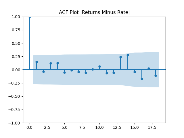
First, we simply test them for independent identically distributed Gaussian: Actually, they are. See the three plots below.
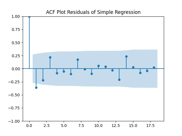
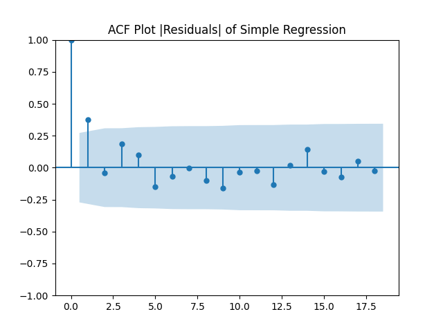
Here is approximate bond duration. We get This is quite similar to the previous research. But unfortunately, residuals are NOT IID Gaussian. See the three plots below.
Then we get and and Student T-test for gives very low but for or we have high p-values, so we fail to reject these null hypotheses. Luckily, these new residuals are, in fact, Gaussian white noise:
The Jarque-Bera and Shapiro-Wilk tests for normality of residuals and which give us high p-values (higher than 10%).
I did this work myself, and I am not sure why results here are so different from the previous two blog posts mentioned at the top of this post. This is left for further research.
A continuation of research in github.com/asarantsev repository Annual-Bank-of-America-Rated-Bond-Data from my previous post. Consider total returns computed from total wealth process as log change: The plot of the wealth process normalized so that is given below. We see that high-yield, low-rated bonds provide more long-run returns but with much more risk.
If these were Treasury bonds and there were no risk of default, and if these were zero-coupon bonds (with only principal payment at maturity) then total returns would be equal to the rate minus maturity times rate change. See my manuscript arXiv:2411.03699. The equation is: If the bonds were having coupons, then instead of maturity there would be duration (average time of coupon and principal payments, weighted by payment size). But we add noise (innovation) terms, and an intercept:
The maturity is given in the following table, together with analysis of residuals: skewness, kurtosis, Shapiro-Wilk and Jarque-Bera normality test valued. Also, we take the sum of absolute values of the autocorrelation function for the first five lags, separately for original values of residuals and for their absolute values.
Rating
Skewness
Kurtosis
Shapiro-Wilk
Jarque-Bera
ACF of
ACF of
AAA
6.03
-2.049
5.173
0.014%
<0.001%
0.539
0.687
AA
4.89
-0.941
1.154
2.549%
5.831%
0.944
0.874
A
4.94
-0.894
1.307
7.877%
5.726%
0.977
0.704
BBB
5.17
-0.573
0.027
25%
46%
0.38
0.604
BB
3.81
-1.75
3.64
0.054%
<0.001%
0.83
0.245
B
3.12
-2.036
4.323
0.003%
<0.001%
1.17
0.653
CCC
2.55
-2.304
5.34
0.001%
<0.001%
0.9
0.716
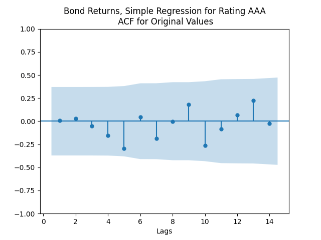
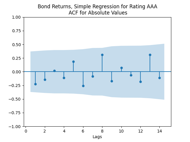
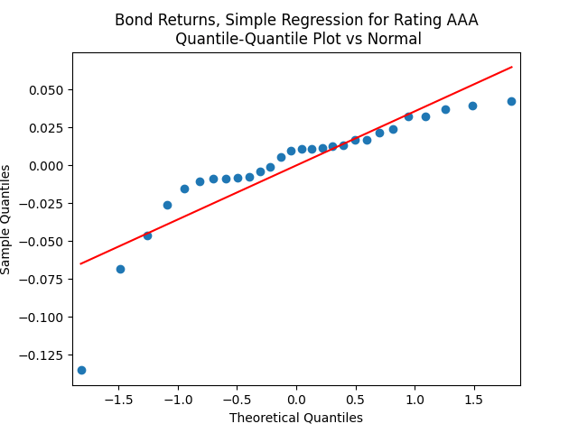
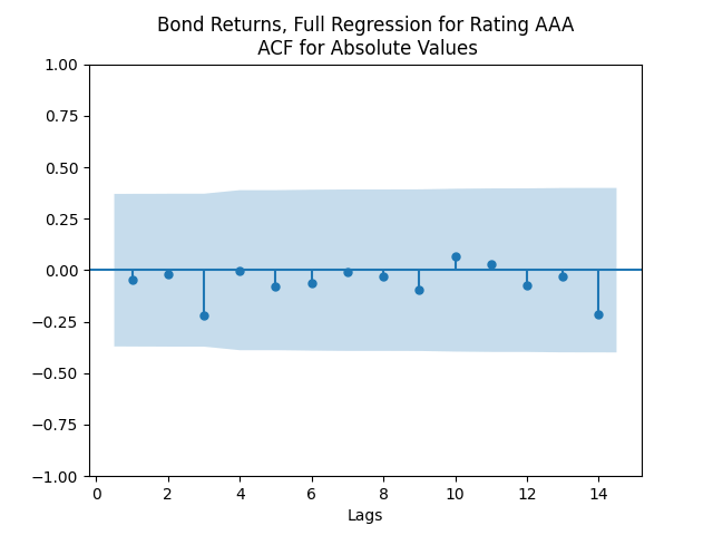
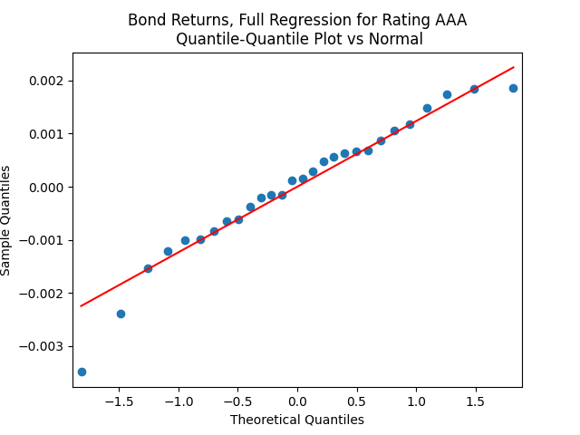
The autocorrelation function plots for and for show that these are independent identically distributed. However, the quantile-quantile plot of versus the Gaussian distribution show these are not normal, for most ratings. See the plots below.
This is confirmed by the results of Shapiro-Wilk and Jarque-Bera tests, shown in the table above.
Apply the same technique as in the previous post: Normalize residuals by dividing them by annual average VIX. We get: We divide this equation by and get an ordinary least squares regression without intercept. This is not usual, so let us add an intercept:
Coefficient estimates and analysis of innovations is shown in the table below.
Rating
Skewness
Kurtosis
Shapiro-Wilk
Jarque-Bera
ACF of
ACF of
AAA
0.0661
7.0787
-0.0034
-0.737
0.576
28%
23%
0.922
0.361
AA
0.0453
5.3226
-0.0023
0.126
-0.039
46%
96%
0.57
0.761
A
0.0423
5.3423
-0.0022
-0.181
0.02
35%
93%
0.73
0.459
BBB
0.0293
5.6074
-0.0016
-0.232
-0.775
67%
62%
0.875
0.498
BB
0.0422
3.6671
-0.0024
-0.894
1.426
19%
6.3%
0.574
0.888
B
0.0682
2.9970
-0.0050
-1.562
3.479
0.397%
<0.001%
0.998
0.354
CCC
0.0712
2.6532
-0.0075
-1.588
2.649
0.072%
0.005%
0.835
0.723
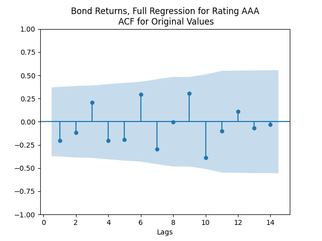
We see the residuals can be well described as Gaussian white noise for ratings BB and higher, especially well for investment-grade bonds. But for B and CCC ratings, not so much. However, judging by the ACF, new residuals (see the second table) are comparable to old residuals (see the first table) in being close to independent identically distributed. See also the following plots for AAA rated bonds:
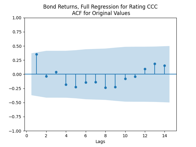
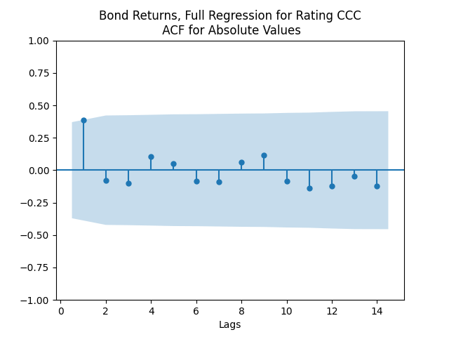
And for the lowest-rated CCC bonds the situation is different: We see that the first lag is quite significant for both version of the autocorrelation function.
Combining the model above with the results of the previous post, we get the trivariate model:
And the wealth process is given by It is possible to show this model for is long-term stable and ergodic, because for each of seven ratings, We have done this for in our previous work. For this is trivial.
Next, for ratings BB and above, the trivariate innovations sequence is modeled as independent identically distributed trivariate Gaussian. Our code find the covariance matrix for these. We do not put it here but an interested reader can run the code.




 We analyze innovations
  for Gaussian IID. Next, we divide
  for annual volatility
  for Gaussian IID.
 Here the
  for the Student T-test. Here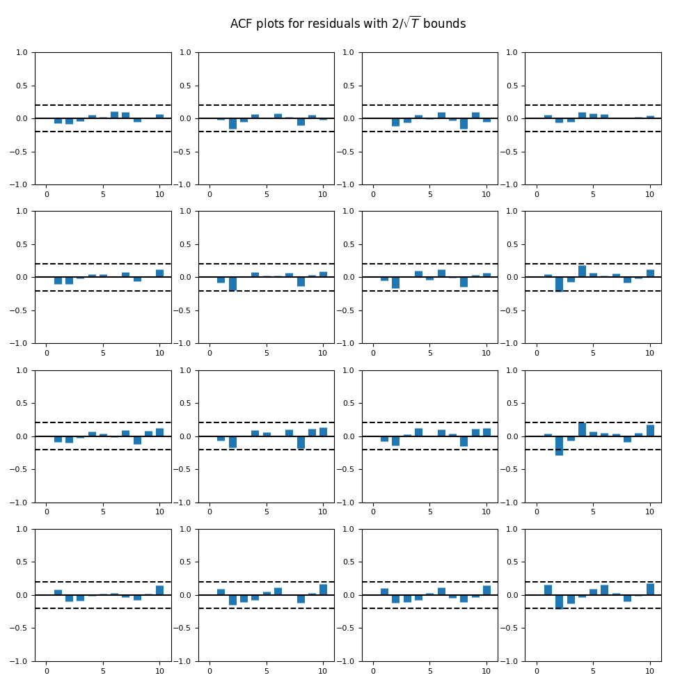
 and
and 
 and
and 
 and
and 
![\mathbf{S}(t) = [S_1(t), S_2(t)]](https://s0.wp.com/latex.php?latex=+%5Cmathbf%7BS%7D%28t%29+%3D+%5BS_1%28t%29%2C+S_2%28t%29%5D+&bg=ffffff&fg=000&s=0&c=20201002) which is BAA-AAA, BAA-Long:
which is BAA-AAA, BAA-Long:
 as independent identically distributed. See below the autocorrelation and cross-correlation plots. The correlation of its two components is 89%.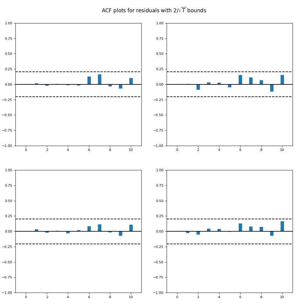
 We see it is reasonable to model
 We see it is reasonable to model
  as independent identically distributed normal.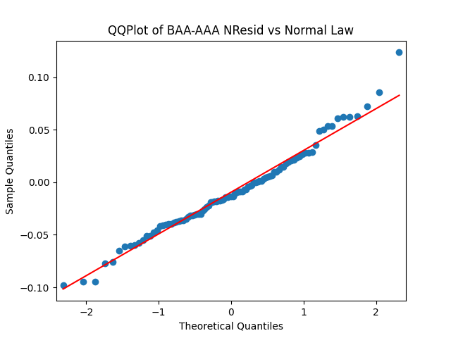




 we need earnings from years
  To get earnings yield for year
  we need earnings from years
  And so on for subsequent years. Thus we need all earnings for each of the last 10 years to be able to simulate returns from this year.
 for all four types of returns. Thus we might state that the 10-year averaging improves the model. However, the
  values are of the same order: around 20-30%.

 with mean zero. Let us write these equations explicitly. Let
  and
and  Let
Let  be the end of year
  be total returns for this index, including dividends. Then we have:


 are significantly different from zero. In particular, returns and volatility have significant negative dependence. But
  is not significantly different from zero. Interestingly, we see that dependence of returns upon earnings yield is positive (undervalued markets grow faster) but very weak. A better measure might be cyclically adjusted price-earnings ratio, called Shiller CAPE, see future posts. This ratio is based on 10-year trailing averaged inflation-adjusted earnings.


 The Shapiro-Wilk tests for nominal and real earnings growth give us
  and
and  We pick the regression for total real returns. Evidence for IID is there but there are problems with this. We are not sure why there is large autocorrelation with lag 4. We did not apply the Ljung-Box omnibus test for the first 5 or 10 autocorrelation values. But we think it would reject the white noise hypothesis. Other regressions for other returns: price real, total nominal, price nominal, show similar autocorrelation plots for residuals and their absolute values.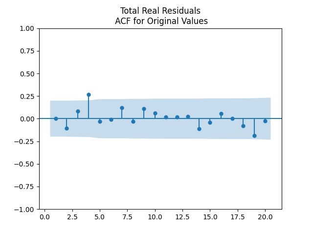

 Note that the log change in earnings yield can be represented as the difference between price returns and earnings growth:

 depends on
  exponentially. This might lead to volatile fluctuations, especially when the yield is large. Then fluctuations are also large. This needs to be researched further.
 as IID, judging by the ACF plot for
 for
for 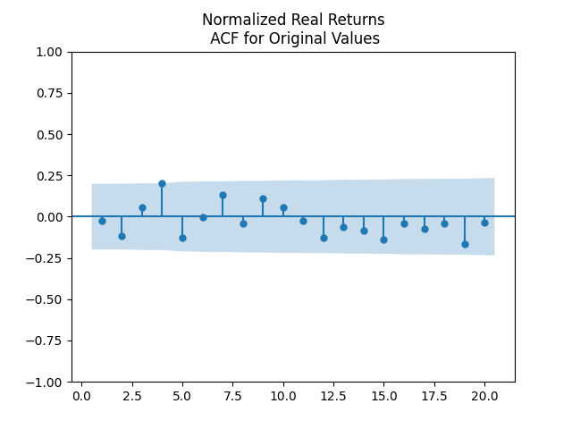

 as bivariate normal IID:
  We found the mean vector and the covariance matrix, for both real and nominal versions. This is available when we run the code.
 This formula would be true for the case when there are no contributions or withdrawals. If each year we have flow (inflow or outflow)
  (positive or negative), then the wealth process is

 in years

 time points, except for volatility, which has
  data points. It is taken from
 for large stocks (measured by top 30%); and
  for small stocks (measured by middle 40%). These are nominal (not inflation adjusted). To adjust them for inflation, we need to subtract monthly inflation rate, computed from the (not seasonally adjusted)

 are independent identically distributed innovations with mean zero.
 as follows: Remove 12 outliers from the 461 in the right tail and model the rest as normal with mean and standard deviation
  and
and  Thus innovations are modeled as a mixture with weights
  of the uniform distribution upon these 12 outliers, and the above normal distribution. We use kernel density estimation to simulate innovations, with Gaussian kernel and bandwidth derived from the Silverman rule of thumb. In this case the bandwidth is 0.03619. This


 are independent identically distributed trivariate Gaussian innovations,
 where
where  are, in fact, IID Gaussian.
  upon
upon  where we take rate data for January of year
 and the Student T-test gives us
  . It seems we can model this rate using random walk. The problem of the random walk model is that it is not stable (ergodic) in the long run. The innovations
  are well modeled as independent identically distributed Gaussian white noise: See the plots below.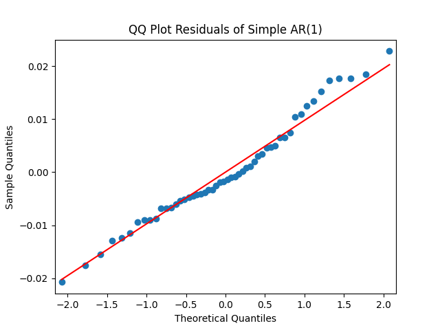
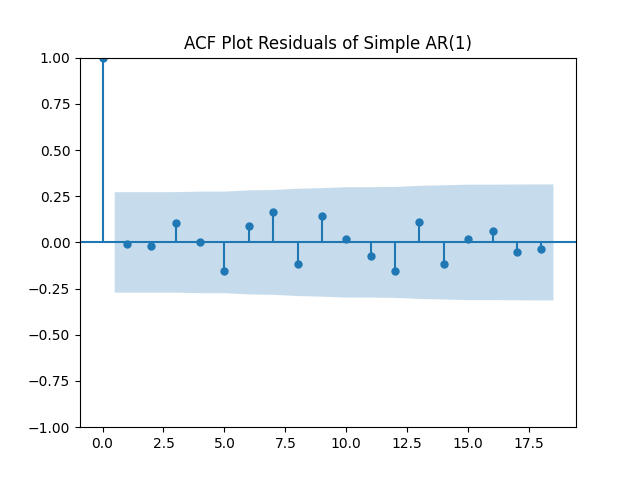
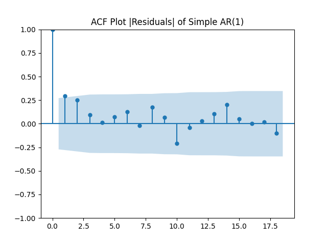
 as follows:
  The mean and standard deviation of these terms are
  and
and 
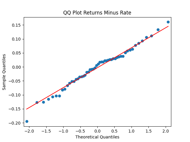
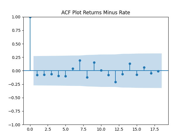

 is approximate bond duration. We get
  This is quite similar to the previous research. But unfortunately, residuals
  are NOT IID Gaussian. See the three plots below.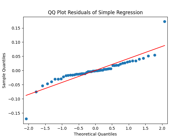

 and
and  and
and  Student T-test for
  gives very low
  but for
  or
or  we have high p-values, so we fail to reject these null hypotheses. Luckily, these new residuals are, in fact, Gaussian white noise: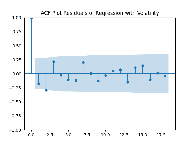
 The plot of the wealth process
  is given below. We see that high-yield, low-rated bonds provide more long-run returns but with much more risk.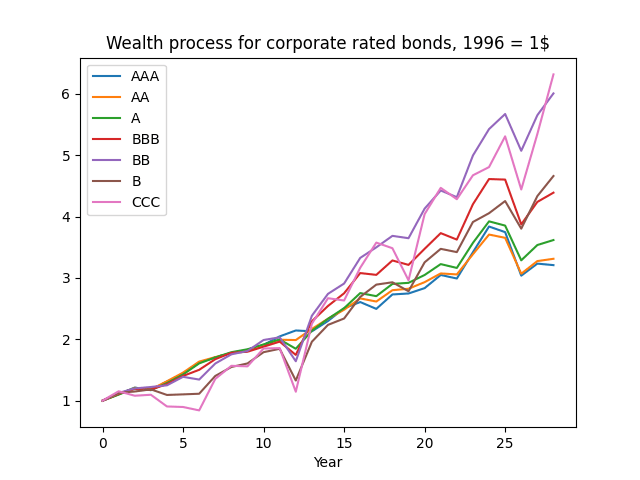
 If the bonds were having coupons, then instead of maturity there would be duration (average time of coupon and principal payments, weighted by payment size). But we add noise (innovation) terms, and an intercept:

 We divide this equation by




 It is possible to show this model for
  is long-term stable and ergodic, because for each of seven ratings,
  We have done this for
  in our
  this is trivial.
 is modeled as independent identically distributed trivariate Gaussian. Our code find the covariance matrix for these. We do not put it here but an interested reader can run
