Updates for 2025

Dear readers, after a long break, I am back. I updated the annual volatility and other data for S&P 500 for the year 2025. The data are available here.

Data Updates
New Graphs
Total Returns
Volatility Autoregression
Price Returns
BAA Bond Rates
Dividend Growth
Conclusion

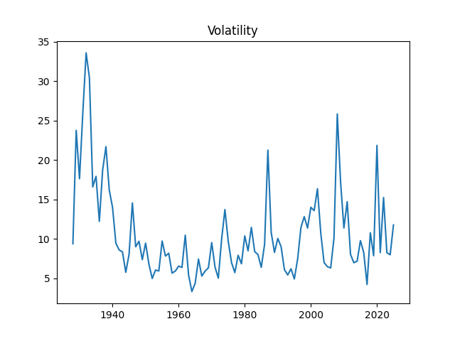
1. Data Updates. Annual volatility is computed as the empirical standard deviation of daily log changes multiplied by 1000 (for normalizing). The end-of-year price for S&P 500 in 2025 is also updated. We also add S&P 500 dividends for 2025. Now we have data on volatility for 1928-2025, on dividends for 1927-2025, and end-of-year level of S&P 500 for 1927-2025 too.

We added the dividend data for 1927 as well, to increase the number of data points. This is fine, since S&P 90 (a predecessor for S&P 500) was created in 1926, and the data is taken from Robert Shiller’s data library.

The volatility for 2025 is 11.77. This is higher than the long-term average 10.51, or the 2024 volatility, which is 7.98. See the original post with computations of Angel Piotrowski for 1928-2023 and its previous update for 2024.

Dividends for 2025 are 78.92, which is significantly higher than dividends for 2024, which are 74.83.

The S&P 500 increased a lot in 2025: End-of-year 2024 level is 5881.63, but end-of-year 2025 level is 6845.5.

We could not yet provide earnings for 2025, since we have earnings for 2025 Quarter 4 reported only on 2026 Quarter 1, which is still ongoing. We will provide them as soon as we can.

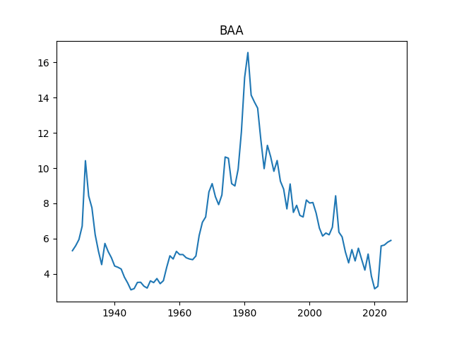
Finally, we added the BAA rate: December 2025 daily average. The BAA are lowest-rated investment-grade corporate bonds. The rate in December 2025 is 5.9, slightly higher than 5.8 for December 2024.

2. New Graphs. We graph the index, dividend, rates, and volatility.

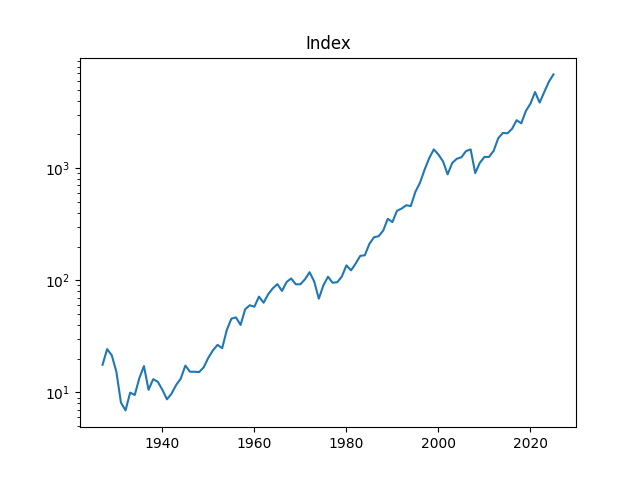
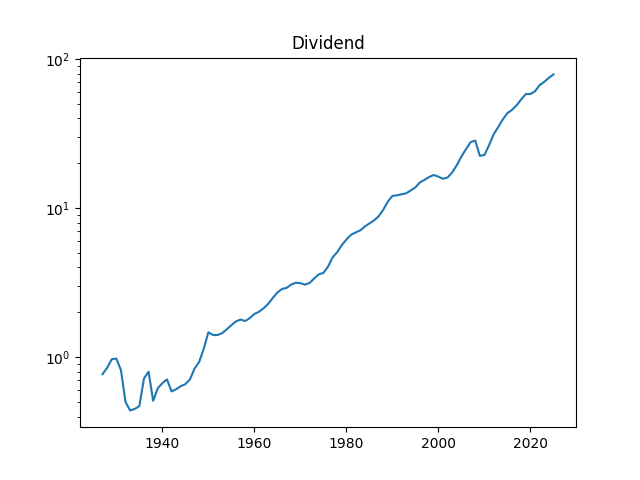
Above, logarithmic plots of index levels and dividends for 1927-2025. Below, the annual volatility and December BAA rate.

The data are published on my web page: We created a new tab named Financial Data Library on my web page. Let us now apply

Let us replicate this post: Make stock returns IID Gaussian.

We have the following notation:

$S(t)$ the S&P level at end-of-year $t.$
$D(t)$ the dividend of S&P in year $t.$
$R(t)$ December daily average BAA rate during year $t.$
$V(t)$ annual realized volatility for the S&P for year $t.$

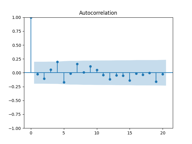
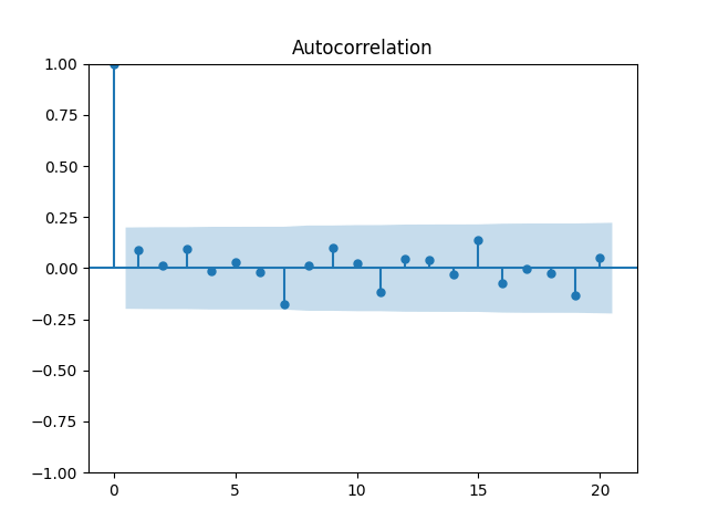
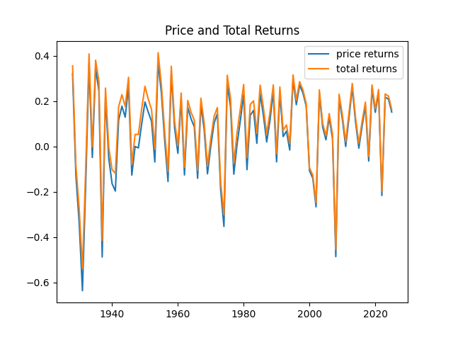
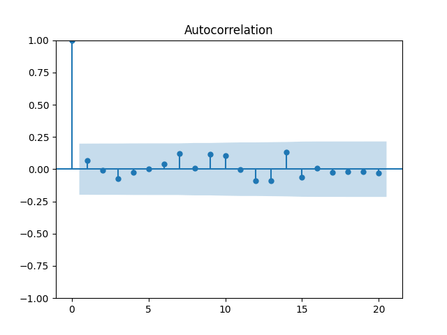
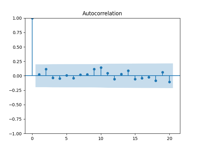
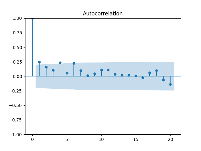
3. Total Returns. We continue this blog post. Compute total nominal geometric returns for the S&P 500: $Q(t) = \ln(S(t) + D(t)) - \ln S(t-1)$ for year $t.$ Below is the graph of returns 1928-2025.

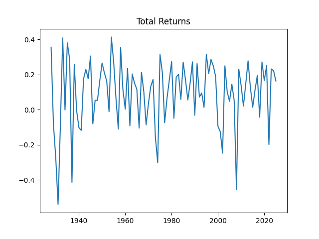
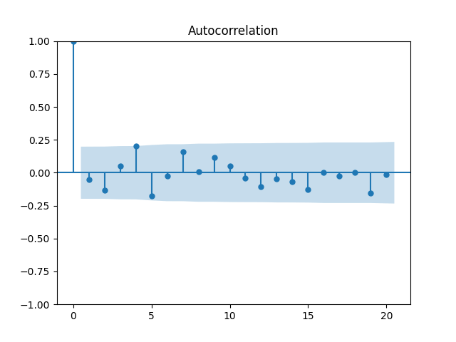
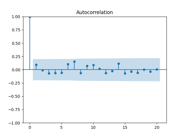
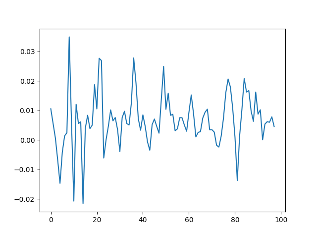
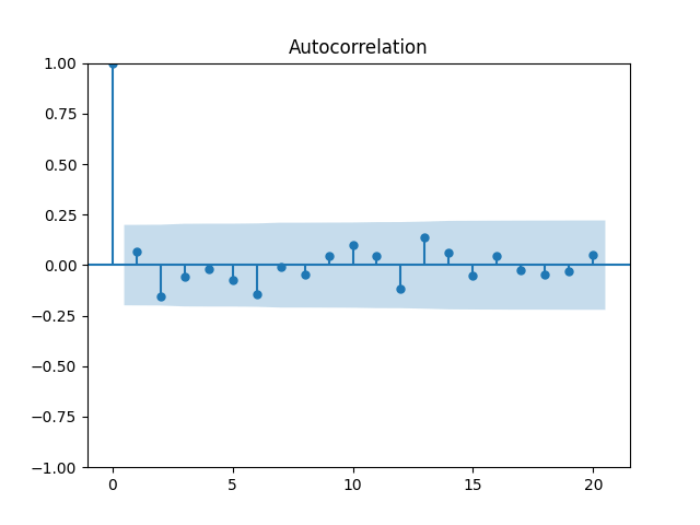
Now plot the autocorrelation function for these total returns $Q.$ And another autocorrelation function for their absolute values $|Q|.$ Both plots are below, and both are consistent with the white noise hypothesis. It is surprising that we, in fact, do not have to divide total returns by annual volatility to make it white noise.

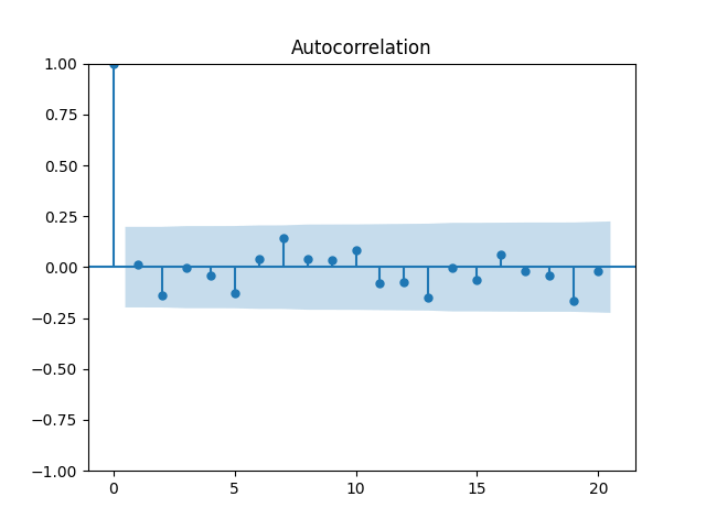
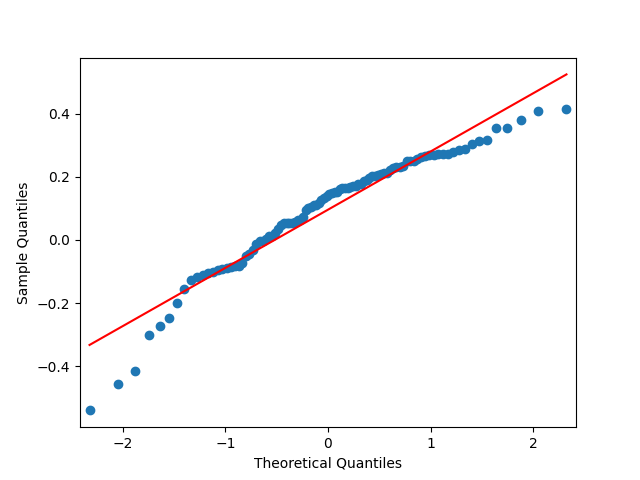
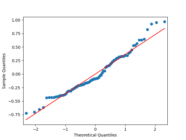
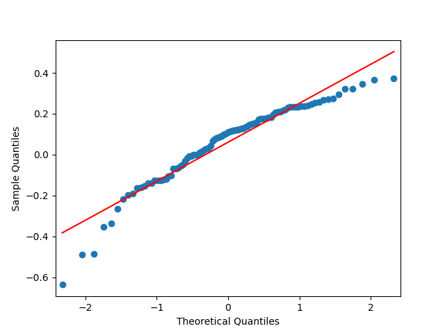
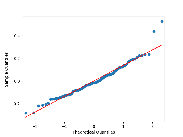
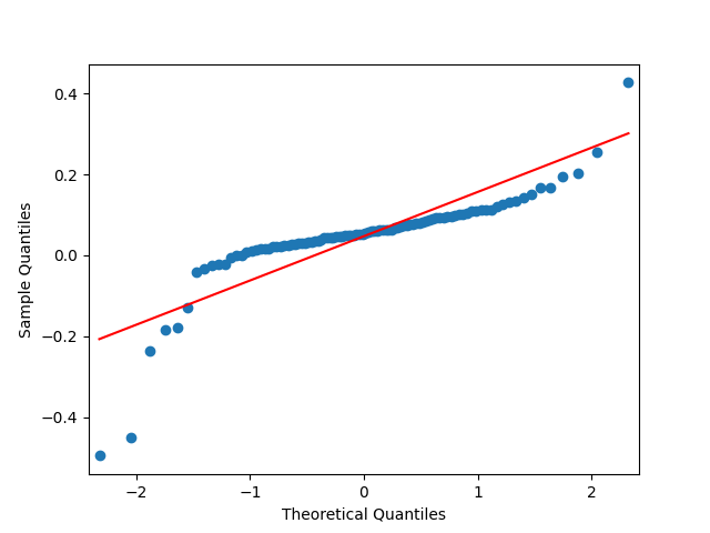
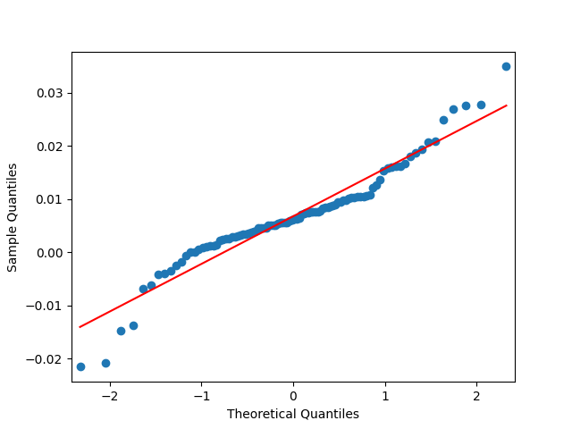
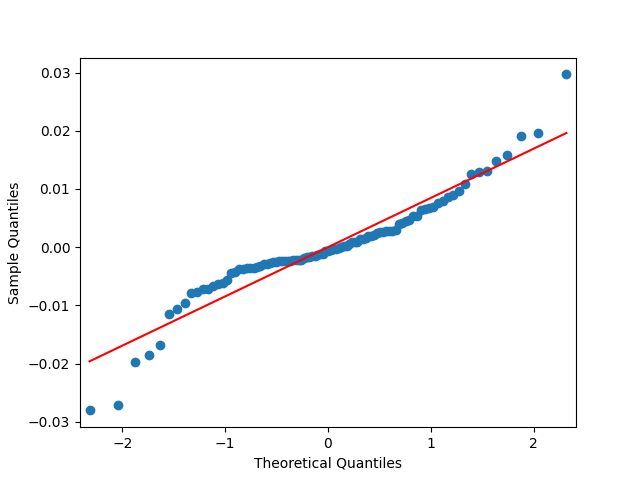
The quantile-quantile plot of these returns is shown as well. We see that the returns are not Gaussian. This is consistent with the normality testing. Shapiro-Wilk and Jarque-Bera tests give us $p = 0.02\%$ and $p = 3\cdot 10^{-5}.$

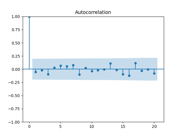
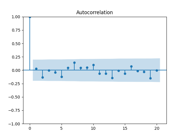
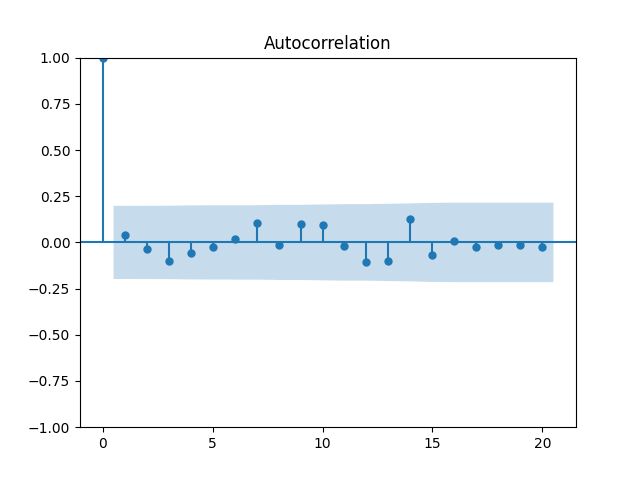
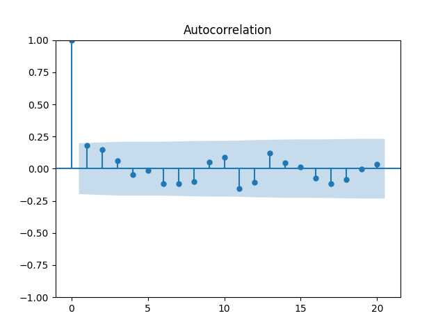
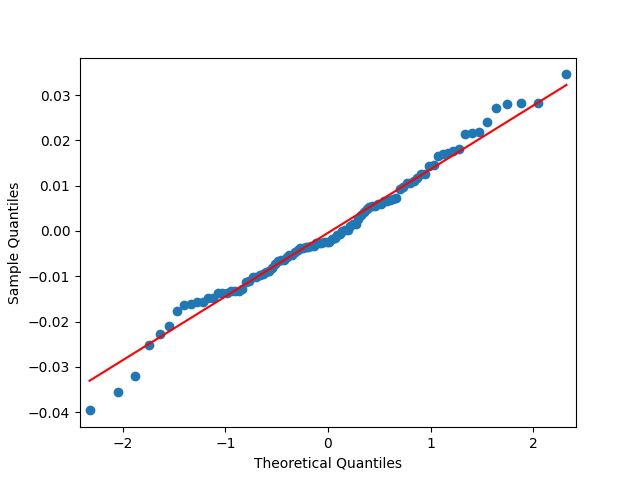
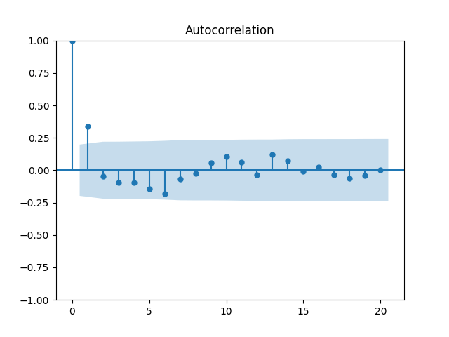
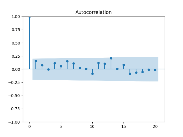
What if we do divide these total returns by annual volatility? We get $N(t) = Q(t)/V(t).$ Let us plot the autocorrelation function for $N$ and the autocorrelation function for $|N|.$

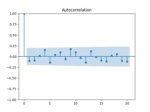
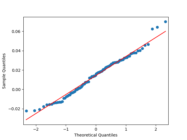
These are still consistent with white noise, although, in my view, the autocorrelation function values are greater. But the quantile-quantile plot versus the normal distribution is below. We get $p = 12\%$ and $p = 71\%$ for Shapiro-Wilk and Jarque-Bera normality tests.

4. Volatility Autoregression. We continue this blog post. Let us now fit the auto-regression model for logarithm of volatility:

$\ln V(t) - ln V(t-1) = \alpha + \beta \ln V(t-1) + W(t).$

We fit $\beta = -0.3824$ and $\alpha = 0.8569.$ Also, plotting the autocorrelation function of $W$ and of $|W|$ we see:

This is consistent with the assumption that $W(t)$ are independent identically distributed. But it is more ambiguous to assume they are Gaussian, see the quantile-quantile plot below. The Shapiro-Wilk and Jarque-Bera tests give us $p = 1.1\%$ and $p = 7.5\%$ respectively.

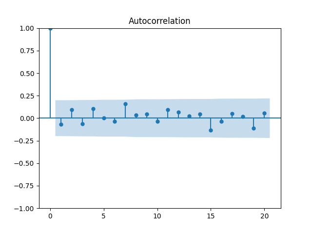
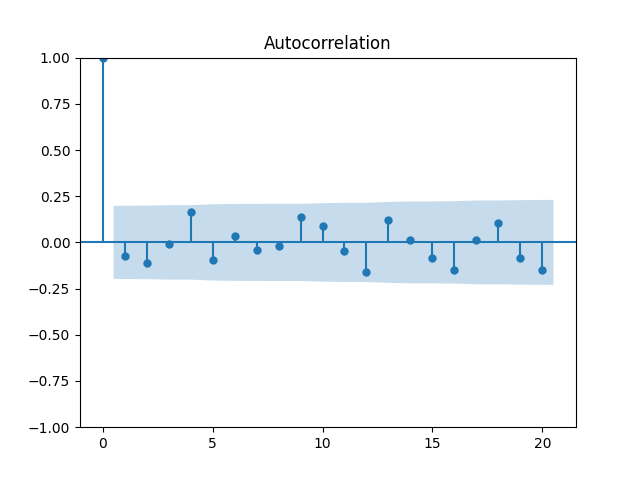
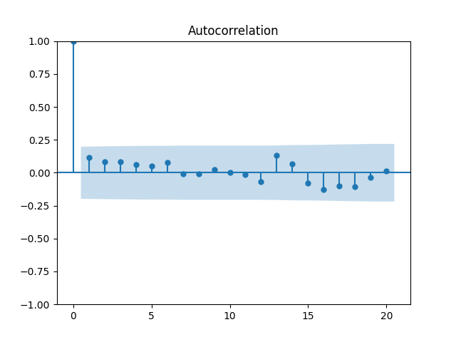
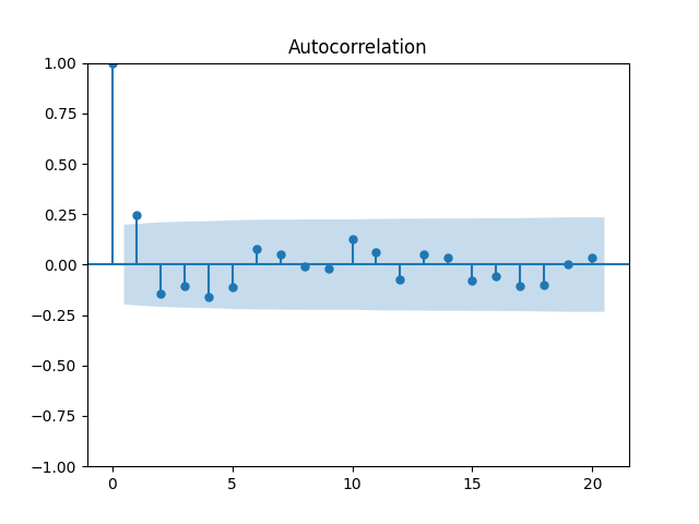
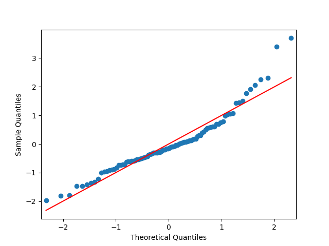
5. Price Returns. These are computed as $Q(t) = \ln S(t) - \ln S(t-1).$ We continue this blog post. These contain only price changes, not dividends. The autocorrelation function for these values and their absolute values is plotted below.

Quite close to independent identically distributed! Next, the quantile-quantile plot versus the Gaussian distribution: This shows price returns are not Gaussian, similarly to total returns. This is confirmed by familiar Shapiro-Wilk and Jarque-Bera tests $p = 7\cdot 10^{-5}$ and $p = 1.4\cdot 10^{-6}.$

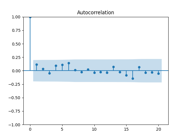
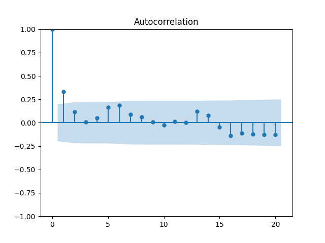
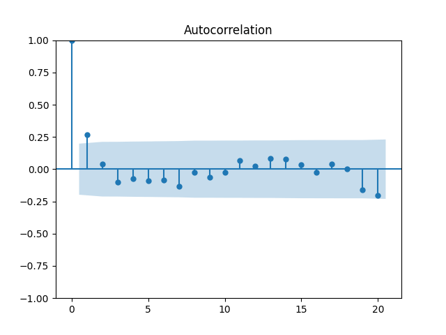
Let us divide price returns by volatility. Below we plot the autocorrelation function of $Q/V$ and of $|Q/V|$ and see that this is still consistent with being independent identically distributed. Only these values are slightly higher.

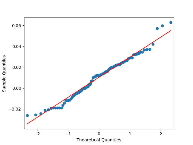
The Shapiro-Wilk and Jarque-Bera tests give us $p = 9\%$ and $p = 75\%$ respectively. See also the quantile-quantile plot. This is much closer to normal distribution.

Finally, let us plot price and total returns together. We see that, of course, total returns are greater than price returns.

6. BAA Bond Rates. Continue this blog. We also fit a simple autoregression:

$R(t) - R(t-1) = a + bR(t-1) + Z(t).$

We get: $a = 0.43$ and $b = -0.062.$ But the p-value for the null hypothesis when we have a random walk is $p = 8\%$ so we fail to reject the random walk hypothesis. This is not acceptable from the financial point of view, since the random walk implies $R$ will go negative eventually. Also, consider the graphs of autocorrelation function for $Z$ and for $|Z|.$ These are not independent identically distributed.

Both p-values for normality tests of innovations $Z$ are less than 0.01%. The quantile-quantile plot is shown below for $Z.$ It is clear these are not Gaussian.

Instead, like for the volatility, let us take the logarithm:

$\ln R(t) - \ln R(t-1) = a + b\ln R(t-1) + Z(t).$

We get $a = 0.11$ and $b = -0.058$ with $p = 9.2\%$ for the null hypothesis of random walk, which corresponds to $b = 0.$ Plot the autocorrelation function for $Z$ and for $|Z|$ below:

Let us modify this to try a random walk model: $L(t) = \ln R(t) - \ln R(t-1)$ are they really independent identically distributed Gaussian? Below are the autocorrelation function plots for $L$ and for $|L|$ which show that these are independent identically distributed.

Next, the quantile-quantile plot versus the normal distribution is much closer to the straight line than before for other models of the BAA rate. This is confirmed that the Shapiro-Wilk and Jarque-Bera tests give us $p = 0.4\%$ and $p = 10^{-5}$ which rejects the null hypothesis but are not as small as the previous ones.

Next, try to make these independent identically distributed but non-Gaussian terms Gaussian. We do the same as in sections 1 and 3: Divide the log rate change by volatility. We get $N(t) = L(t)/V(t) = \ln(R(t)/R(t-1))/V(t).$ Below are autocorrelation function plots for $N$ and for $|N|.$

The quantile-quantile plot below shows these are Gaussian terms, and the same is shown by the Shapiro-Wilk and Jarque-Bera tests with $p = 46\%$ and $p = 91\%.$ This was done in the spirit of this blog post.

7. Dividend Growth is computed as $G(t) = \ln D(t)/D(t-1).$ We continue this blog post. See below the autocorrelation function plots for $G$ and for $|G|$ which show lag 1, also the quantile-quantile plot.

Define $N(t) = G(t)/V(t)$ and analyze it as well. The data are closer to the Gaussian distribution, with $p =0.03\%$ and $p = 0.01\%.$

See the plot of the dividend growth below. It is quite volatile but not as much as the stock returns. But we clearly see the persistence: It makes sense to model dividend growth or its normalized version as the simple autoregression. This is different from annual earnings growth, where dividing by volatility makes it independent identically distributed, see this blog post.

Let us try the simple autoregression for normalized annual dividend growth $N(t) = \ln(D(t)/D(t-1))/V(t).$

$N(t) - N(t-1) = k + mN(t-1) + Y(t)$

We have $k = 0.0044$ and $m = -0.66$ with $p < 10^{-9}.$ Shapiro-Wilk and Jarque-Bera normality tests give us $p = 6\cdot 10^{-5}$ and $p = 1.7\cdot 10^{-7}.$ See the graphs below, autocorrelation for $Y$ autocorrelation for $|Y|$ and the quantile-quantile plot for $Y.$

Here we have independent identically distributed but not Gaussian residuals $Y.$

8. Conclusion. Here, we found all time series Markov models for dividends, price and total returns, volatility, and the BAA rates. In the next post, we will discuss updates for the valuation measure based on one-year dividends instead of trailing 10-year earnings, and regression modeling using rate change and duration, continuing this post and this post.

Responses

New Valuation Measure based on Dividends – My Finance

January 30, 2026 at 9:38 pm

[…] continue the previous blog post. We replicate the valuation measure here. Previously we did this with 10-year earnings but now we […]

LikeLike

Bond Returns 1973-2025 – My Finance

February 2, 2026 at 10:36 pm

[…] the research after updating the data for 2025. In the previous post, we discussed total returns for S&P 500 in detail. Now we […]

LikeLike

Updates for 2025

Share this:

Responses

Leave a comment Cancel reply