My Finance

Introduction. Here I talk about improvement of my financial simulator. So far, I have the following factors:

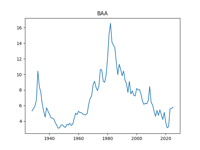
• BAA corporate bond rate, average December
• Annual volatility, S&P 500

I decided to include two more important factors:

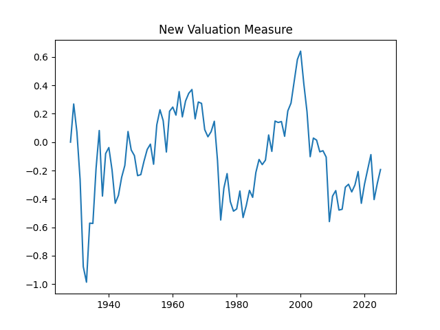
• A bubble measure, which is an improvement over Robert Shiller’s cyclically adjusted price-earnings ratio (CAPE), for which he got a Nobel Prize in Economics. We discussed it here and here and here.
• The long-short spread between 10-year and 3-month (average December) Treasury rates, which is often quoted as an important indicator. For example, if it is negative (inverted yield curve), then a recession is looming. We discussed it here and here and here.

We will now use annual earnings of S&P for our research. This is important, since it connects stock returns with fundamentals. This is similar to computing bond returns using bond rates. Robert Shiller used this comparison for his work. And we use this comparison to make our valuation measure. But, of course, stocks are much more volatile than bonds. So it’s harder to model.

Since we covered so much in previous posts, here we will be brief. For the person who wants to know details, we refer to GitHub repository.

Results. 1. First, recall the autoregression of order 1 for annual volatility:

Recall that

2-3. Then, modify the autoregression for log BAA rate to include spreads: This is vector autoregression of order 1:

It does NOT include volatility. It has intercept and the slope matrix

4. Model annual earnings by considering its growth: We model this as a regression

As usual, we fit it after dividing by volatility. We have

5. Next, we consider the bubble measure computed as in the above blog posts, with 10-year averaging window, and without using volatility. We get for and

6. We fit the corporate bond returns (geometric) denoted by in the same way as above. Namely,

This makes sense in the context of bond markets, even though we use geometric instead of arithmetic returns here. Note that this does not use volatility. Similar to the above post, we see:

7. Next, we fit the geometric Standard & Poor 500 returns by dividing it by volatility We also do regression versus

The quantity plays the role of the duration: Dependence upon the change in interest rates. This coefficient is negative because returns of stocks and bonds decrease when interest rates increase. Next, is the coefficient for the bubble measure. Of course, this is also negative, since being in a bubble implies low future returns. Same is true for the long-short spread, as discussed at the top of this post. Numerical values of coefficients are:

8. Finally, for international stocks we do the same. Thus we write this regression as

Note that is still the duration. Although is BAA rate, which is the USA, but it influences the international stocks as well. Same for the bubble measure. Numerical values of coefficients are:

Remark. In the regression for earnings growth, we tried instead of , but the p-value for the Student test is too large. Also, we tried instead of , but the p-value for the Student test is too large. We used covariates in linear regressions if Similarly, for the international stocks, we found that spread is not statistically significant.

Innovations. Thus we have 8 (eight) innovation series. Only for can be modeled as Gaussian. But all of them, judging by the autocorrelation function for and for and other tests, can be modeled as independent identically distributed random variables.

I do not have energy to present all these plots for each innovation series. But below is the table. Here, ACF is the L1 norm for the first 5 lags of the autocorrelation function values. Kurtosis is normalized so for normal distribution it is zero. Of course, the same is true for skewness.

Series	Length	Skewness	Kurtosis	Shapiro-Wilk p	Jarque-Bera p	ACF original values	ACF absolute values
Volatility	96	0.401	0.401	0.401	0.401	0.401	0.237
BAA rate	97	0.008	1.754	0.008	0.002	0.375	0.655
Long-short spread	97	1.058	3.382	0.000	0.000	0.455	0.468
Earnings growth	97	0.614	2.903	0.000	0.000	0.474	0.253
Bubble measure	97	-0.816	1.102	0.003	0.000	0.291	0.608
US corporate bond returns	52	0.193	0.238	0.857	0.800	0.878	0.706
US stock returns	97	0.039	0.157	0.344	0.940	0.413	0.590
International stock returns	55	-0.015	-0.202	0.941	0.953	0.527	0.331

Covariance matrix

Correlation matrix

See below the p-values for the Student T-test for null hypothesis which is zero correlation between series of innovations.