My Finance

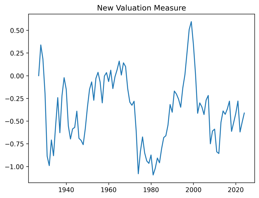
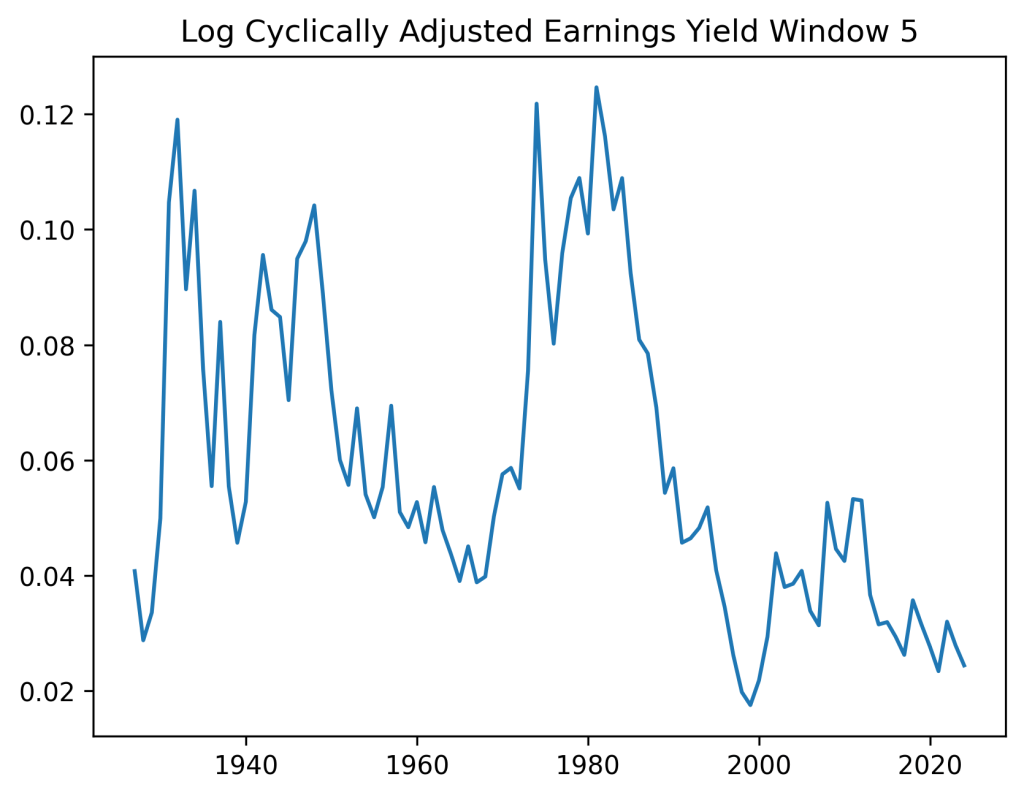
In this post, we regress annual total real returns of S&P 500 vs both new valuation measure and the cyclically adjusted price-earnings ratio (Shiller CAPE) with averaging window of 5 or 10 years. We also use, as usual, the annual volatility. Instead of this Shiller CAPE, we use its inverse, which we call simply the yield. We call the new valuation measure the bubble. We use the version of this new valuation measure at the end of that post. See GitHub/asarantsev repository https://github.com/asarantsev/New-Valuation-Measure-Replication file compare-bubble-logyield.py

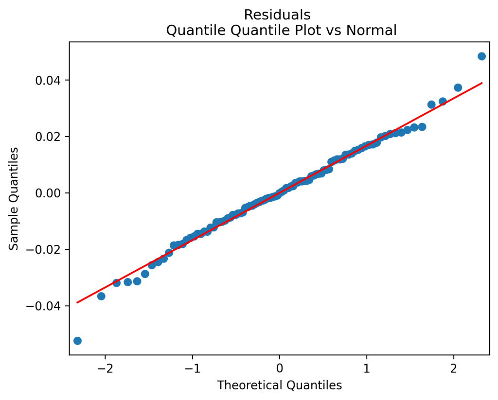
The total real returns are regressed upon the bubble and the log yield end of last year. The residuals of this regression are also normalized by volatility, so we again divide the regression equation by volatility. This time, we do add an intercept, which becomes the volatility factor. Results are as follows: the autocorrelation plots of residuals and their absolute values show that these residuals are IID, see below. The quantile-quantile plot shows these are Gaussian. Same from normality tests.

The dependence of returns upon the bubble is negative (as expected) and strong, with The dependence upon the (log) yield is, surprisingly, also negative but weak, with The dependence upon volatility is negative and very strong, with The

What if we remove the yield? The new is almost unchanged, and the adjusted version is even greater after removal. This shows superiority of the bubble upon the yield as predictor.

On the other hand, removing the bubble instead of the yield reduced and the yield factor becomes a positive predictor of total returns, but statistically insignificant, with

Finally, removing both bubble and (log) yield reduced which is not much below.

The same results are for the window 5 instead of 10.

To me, it makes sense to use either yield or bubble, but not both. This applies to the model without any other factors, or with bond spreads, or something else.