My Finance

See the GiHub repository https://github.com/asarantsev/growth-spread

Continuing research of Ian Anderson, we model by dividing it by annual volatility Here, is annual (nominal or real) earnings of Standard & Poor 500 and its predecessor Standard & Poor 90. We regress it upon BAA-AAA and BAA-10YTR spreads and studied here. We have data 1927-2024 annual. We take spreads for average daily December values. Consider three possible regressions:

• Model 0:
• Model 1:
• Model 2:
• Model 3:

For each regression, we compute both nominal (not inflation-adjusted) and real (inflation-adjusted) earnings growth. Thus we have 6 models. We compute autocorrelation function plots for each and All these look like white noise. Also, we compute 5-lag L1 norm for autocorrelation function for each of these 6 series of residuals and other 6 series of their absolute values. All these 12 numbers are less than 0.6, which is less than the 95% critical value; see Monte Carlo simulations. The following table shows skewness, kurtosis, and the results of Shapiro-Wilk and Jarque-Bera normality tests.

Series	Skewness (Normal 0)	Kurtosis (Normal 0)	Shapiro-Wilk	Jarque-Bera		p-value for Student test
Nominal	0.479	2.158	0.3%	0.0%	7.2%	32% (volatility)
Real	0.459	1.893	0.7%	0.0%	4.9%	24% (volatility)
Nominal	-0.114	2.105	1.3%	0.0%	4%	5.2% (BAA-AAA) and 6.9% (BAA-10YTR)
Real	-0.136	1.861	2.8%	0.1%	5.2%	5.2% (BAA-AAA) and 6.9% (BAA-10YTR)
Nominal	0.163	2.226	0.6%	0.0%	23.6%	3.4% (BAA-AAA) and 1.4% (BAA-10YTR)
Real	0.137	2.039	1.0%	0.0%	15.4%	1.4% (BAA-AAA) and 0.7% (BAA-10YTR)
Nominal	0.256	2.068	1.2%	0.0%	13.3%	27.4% (volatility)
Real	0.227	1.86	1.9%	0.1%	12.4%	23.8% (volatility)

The quantile-quantile plot of earnings growth (nominal and real) versus the Gaussian distribution for Model 0:

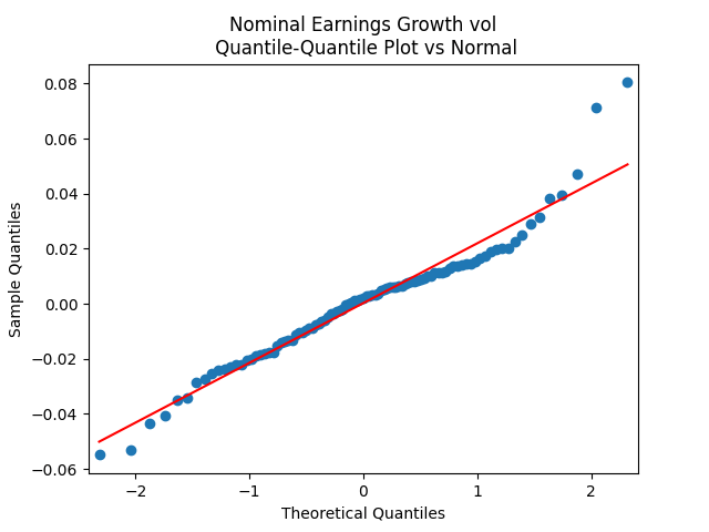
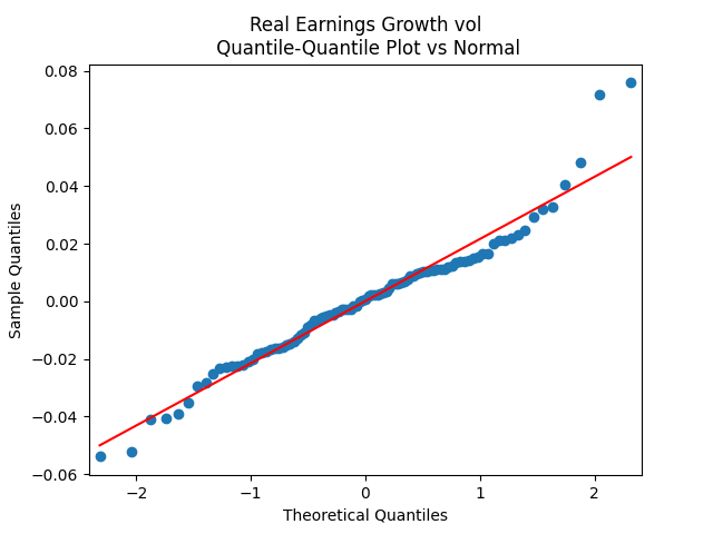
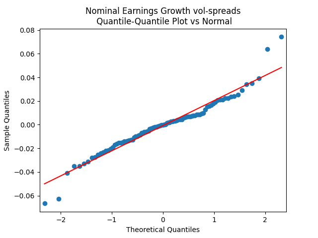
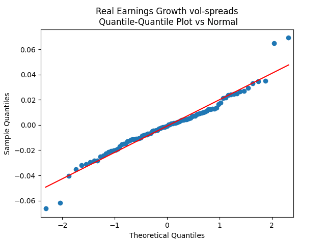
The quantile-quantile plot of earnings growth (nominal and real) versus the Gaussian distribution for Model 1:

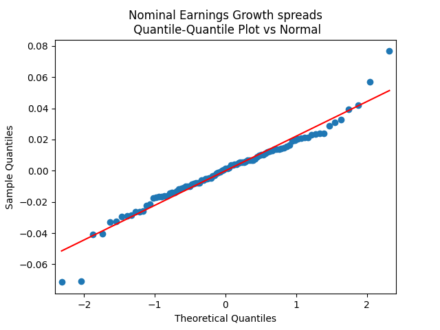
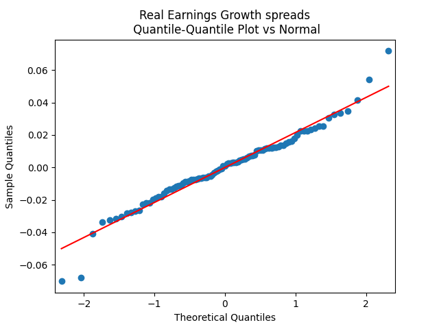
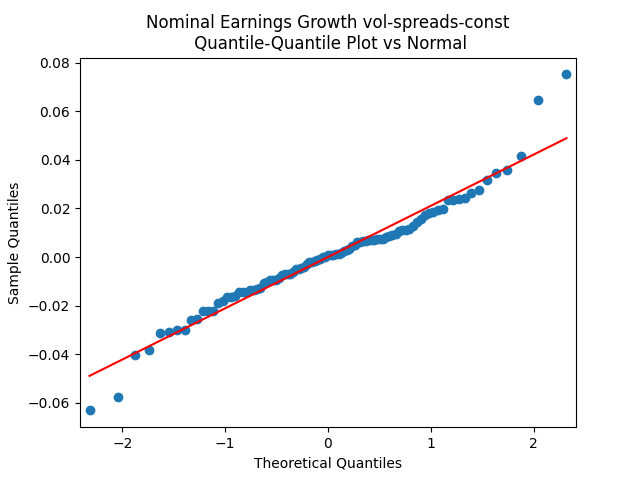
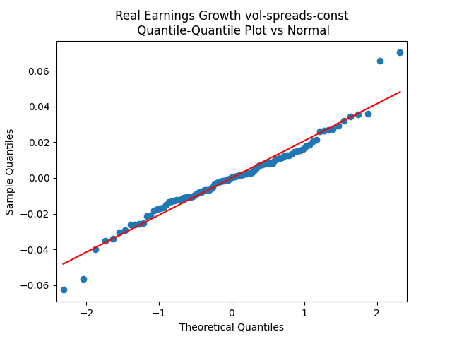
The quantile-quantile plot of earnings growth (nominal and real) versus the Gaussian distribution for Model 2:

The quantile-quantile plot of earnings growth (nominal and real) versus the Gaussian distribution for Model 3:

Conclusion: Unfortunately, residuals are independent identically distributed but not Gaussian, for each of the four models. Still, we need to pick one. Let us pick Model 2: Volatility is not significant, as shown by the Student test. Although it is not quite applicable, since residuals are not Gaussian! Let us write this equation after multiplication by the volatility: