My Finance

In this post, we discuss a version of this financial simulator for annual data. In the last post, we discussed its currently published monthly version. This is a simplified version based on work by Angel Piotrowski. Here we do not have any bond rates or spreads, any earnings or dividends. We have only annual volatility, previously computed by Angel, and total returns data, available on my web page. The code and data are also available on GitHub/asarantsev repository annual-simulator.

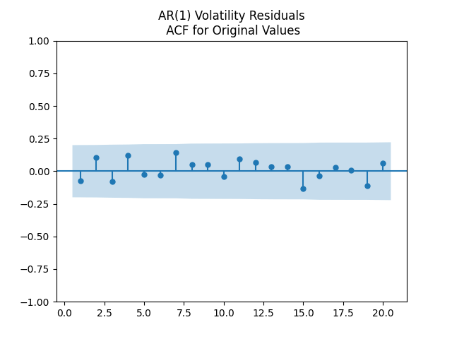
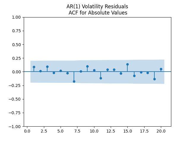
We have log Heston model for annual volatility :

Here, we can model as IID, judging by the ACF plot for and the ACF plot for

It turns out we cannot quite model by a normal distribution. But it is quite close. See also the table below. This is quite weak evidence of normality! Next, we model total (including dividends) real (inflation-adjusted) returns as follows: for IID Gaussian:

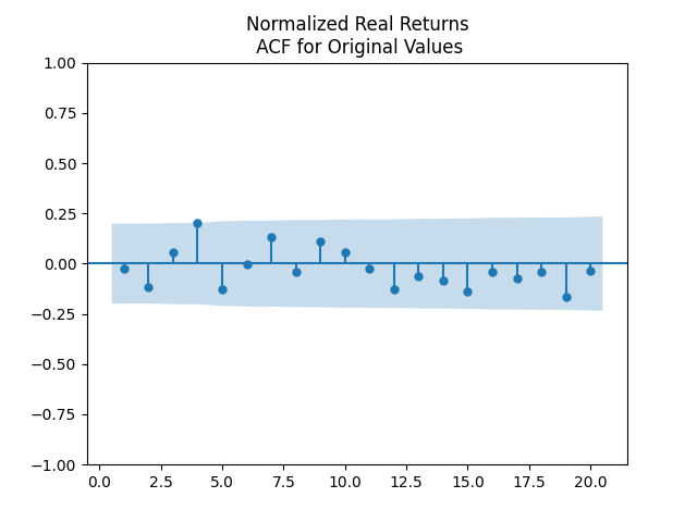
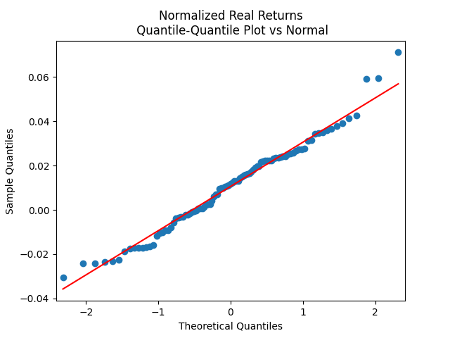
These normalized returns are very well modeled by IID Gaussian. This is confirmed by the plots above. Similar plots are found for the nominal versions of returns.

Data	Skewness (normal =0)	Kurtosis (normal = 0)	Shapiro-Wilk	Jarque-Bera
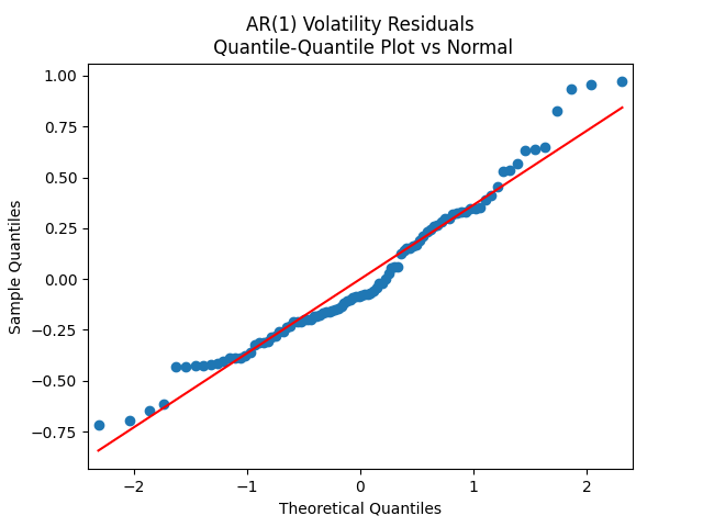
AR(1) Innovations for Log Volatility	0.59	0.057	0.94%	6.1%
Normalized Total Nominal Returns	0.22	-0.21	11%	60%
Normalized Total Real Returns	0.24	0.023	20%	63%

We model as bivariate normal IID: We found the mean vector and the covariance matrix, for both real and nominal versions. This is available when we run the code.

Next, the code has a function which simulates 1000 paths of wealth:

for This formula would be true for the case when there are no contributions or withdrawals. If each year we have flow (inflow or outflow) (positive or negative), then the wealth process is

The arguments of this function are:

1. Choose: Real or Nominal?
2. initial wealth
3. flow each year
4. time horizon in years
5. initial volatility

We rank 1000 simulations by final wealth. This is the same ranking as by average total returns, if only we have no contributions or withdrawals. But if we do have inflows or outflows every year, then these rankings by wealth vs by returns might be different. For each paths, we compute average total returns

We pick simulations corresponding to 10%, 30%, 50%, 70%, 90% ranking of final wealth. We chose these because it gives us more or less comprehensive picture of randomness. It is trivial but often neglected that markets have a lot of volatility. It is not enough to provide mean or median returns or wealth. We need the entire distribution.

One could suggest a histogram of final wealth. But a histogram is hard to read by ordinary users. Also, it shows less information than wealth paths. To laypeople, wealth paths fluctuate wildly, and the path which are on top now can drop fast later. But the histogram does not show that.

Why choose these 5 quantiles? We need to show the median (typical wealth) and the outliers. But one should not go too far. Showing the path corresponding to the maximal or minimal final wealth would give a distorted picture: Users might misunderstand these and think that such outcomes are typical. Even showing the paths corresponding to 5% or 95% final wealth are not very typical: These are outliers, atypical outcomes.

The range of 10%, 30%, 50%, 70%, 90% shows full range of outcomes, but only typical outcomes, not outliers.

We also stress that average final wealth does not mean we exceed this wealth in 50% of simulations. The distribution of the final wealth is much skewed, so mean and median are not the same!

Note than in case of withdrawals, the path might end in ruin (bankruptcy; zero wealth). If some of the chosen five paths has this, we show this and we do not compute average total returns. We also compute average total returns for paths which do not end up in ruin.

We compute how many paths end in ruin, thus the empirical probability of ruin. This is a major problem in retirement planning: How much can we withdraw per year so that we do not end up in ruin? The classic withdrawal rate is 4% (of initial wealth) per year, if we adjust these withdrawals for inflation.

We adapted the Python code for running locally, so it contains a function which makes this plot below. This is quite different from the Python code in the simulator, which includes entering data from a web page and putting the output using this web page. We also have HTML code for this web page. For running this Python code locally, obviously we do not need this HTML page, only the Python code itself.

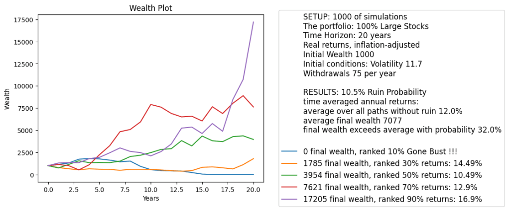
Interestingly, even gigantic 7.5% annual withdrawal rate within 20 years results in only 10.5% ruin probability! Our analysis shows we can be much more permissive with withdrawals than the classic 4% rule.