My Finance

In the two previous blog posts, we considered rates and returns for Bank of America-rated corporate bond portfolios, with ratings AAA, AA, A, BBB, BB, B, CCC. We analyzed annual data and used annual averaged VIX (S&P 500 volatility index) to fit Markov time series models. We were successful: For 5 of these 7 ratings, we created a trivariate model with independent identically distributed trivariate Gaussian innovations. Unfortunately, data was available only starting from 1996. This is less than 30 years.

It would be nice to extend this for a larger time period. We have Moody’s AAA rates back from 1962 (and if you wish only monthly data, all the way from 1919!) But the wealth process (from which we compute total returns) for Bank of America’s corporate bond portfolio is available daily from 1972. To replicate the previous research, we need annual volatility data. But VIX goes only back to 1990, and if we consider volatility for a related index S&P 100, only back to 1986. Thus we need another version of annual volatility. Luckily, Angel Piotrowski provided annual realized volatility for S&P 500 (and its predecessor, S&P 90). This code and data is available on GitHub/asarantsev repository Corporate-Bonds-Annual-Data.

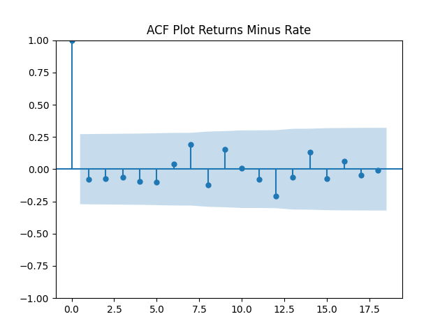
Consider the sequence of rates which in fact can be modeled by a simple autoregression of order 1:

Results: and the Student T-test gives us . It seems we can model this rate using random walk. The problem of the random walk model is that it is not stable (ergodic) in the long run. The innovations are well modeled as independent identically distributed Gaussian white noise: See the plots below.

This is different from the Bank of America AAA rated bond rates, where we needed to include VIX to make innovations normal.

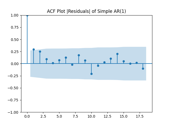
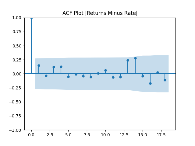
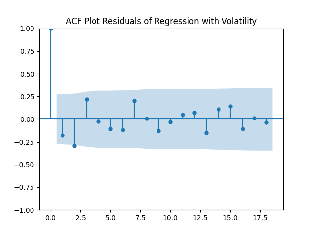
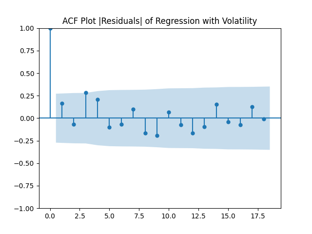
We also ran autoregression including volatility terms as in previous post. We saw that here, the ACF of absolute values of residuals is not white noise.

But let us continue with total returns computed from wealth process as follows: The mean and standard deviation of these terms are and

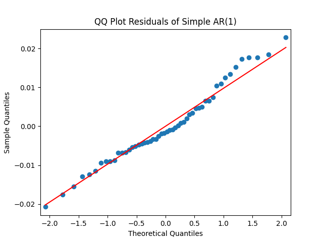
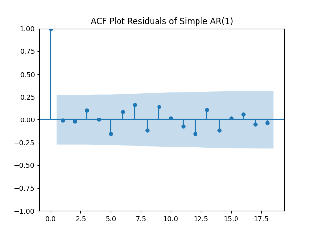
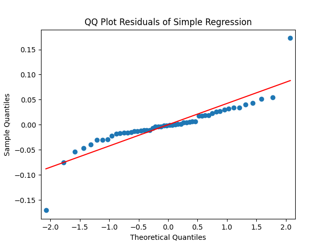
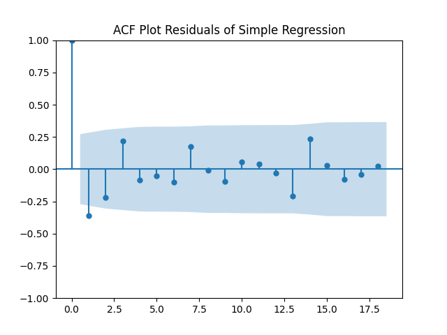
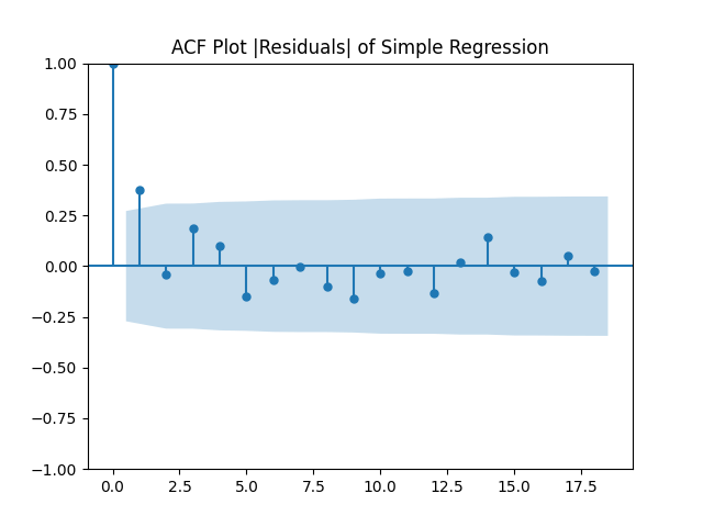
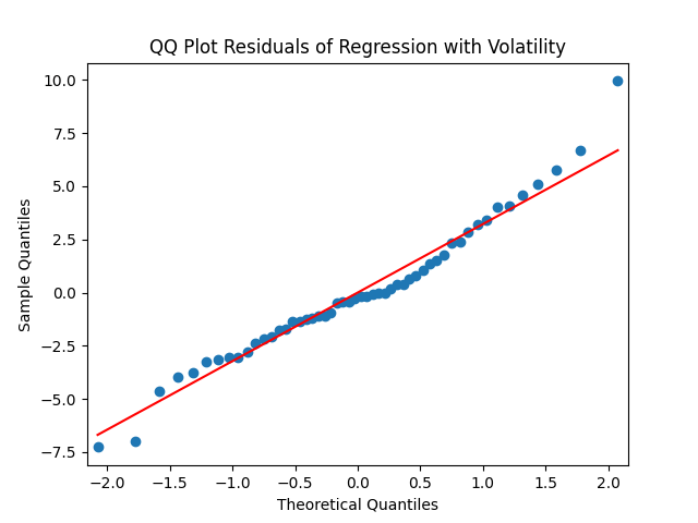
First, we simply test them for independent identically distributed Gaussian: Actually, they are. See the three plots below.

Similarly to Bank of America rated bond portfolio, we write a simple linear regression:

Here is approximate bond duration. We get This is quite similar to the previous research. But unfortunately, residuals are NOT IID Gaussian. See the three plots below.

We know what to do from our previous research: Rewrite this regression as

Then we get and and Student T-test for gives very low but for or we have high p-values, so we fail to reject these null hypotheses. Luckily, these new residuals are, in fact, Gaussian white noise:

The Jarque-Bera and Shapiro-Wilk tests for normality of residuals and which give us high p-values (higher than 10%).

I did this work myself, and I am not sure why results here are so different from the previous two blog posts mentioned at the top of this post. This is left for further research.